9 Cluster Analysis

Author

Pulong Ma

9.1 Learning Objectives

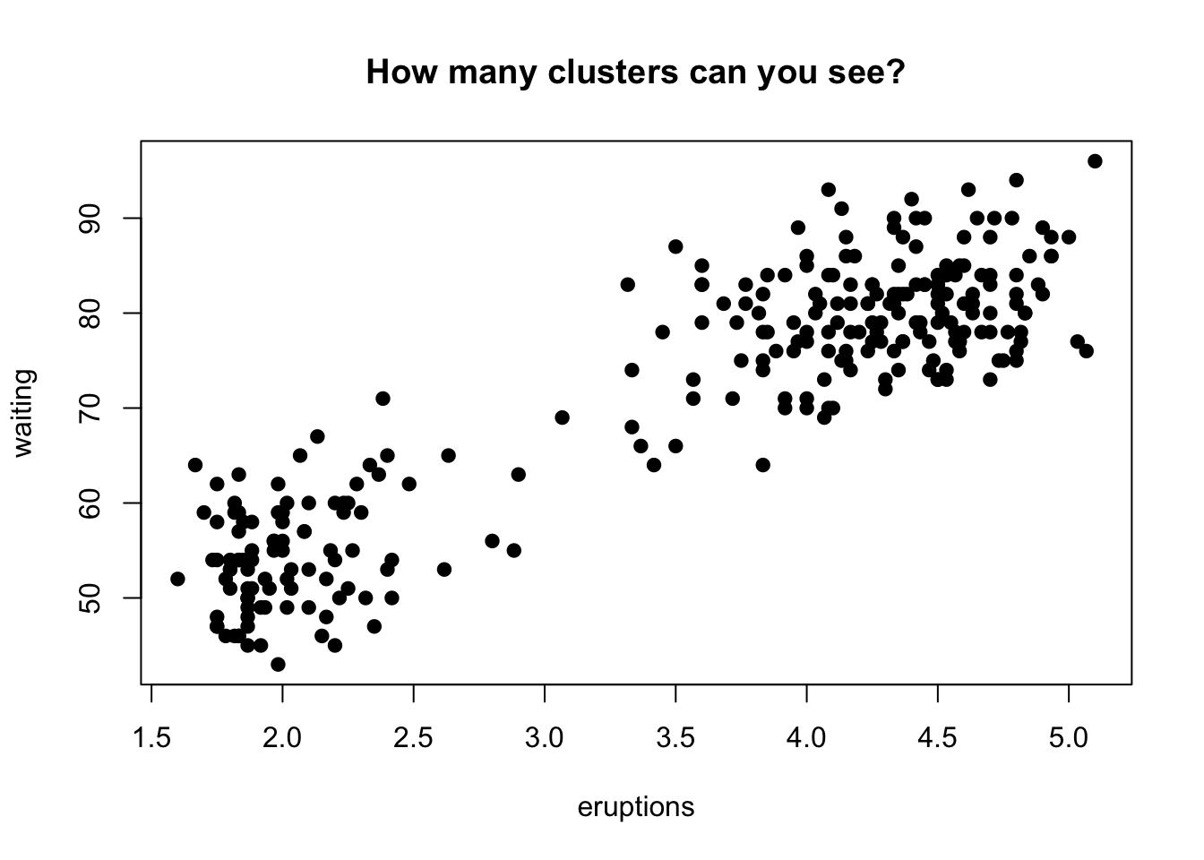
By the end of this lecture, you should be able to:

Explain what cluster analysis is and when it is used.
Distinguish between:
- Hierarchical clustering
- K-means clustering
Compute and interpret distances between observations.
Read and interpret a dendrogram.
Run hierarchical and K-means clustering in R.
Use simple criteria (Calinski–Harabasz index, Gap statistic) to help choose the number of clusters.

9.2 What is Cluster Analysis?

Goal: Discover reasonable groupings (“clusters”) of subjects or units.

Examples:

Group medical patients by how they use different types of services.
Group potential customers by product preferences.
Group environmental habitats by land cover types.
Group foods by nutrient content.

Unsupervised learning

Cluster analysis is an unsupervised learning method:

No response variable / labels.
We only use similarity/dissimilarity between observations.

9.2.1 Clustering Example: Old Faithful Geyser

Data: eruption durations and waiting times.

Code

data(faithful)
plot(faithful,
     main = "How many clusters can you see?",
     pch = 19)

Interpretation

Interpretation:
- There seems to be two groups in the dataset
- Short waiting, short eruption
- Long waiting, long eruption

9.2.2 Data for Cluster Analysis

Big picture:
- n individuals (cases)
- p variables (or traits) measured on each case \mathbf{x}_{1}=\begin{pmatrix} x_{11} \\ x_{12} \\ \vdots \\ x_{1p} \end{pmatrix}, \mathbf{x}_{2}=\begin{pmatrix} x_{21} \\ x_{22} \\ \vdots \\ x_{2p} \end{pmatrix}, \ldots, \mathbf{x}_{n}=\begin{pmatrix} x_{n1} \\ x_{n2} \\ \vdots \\ x_{np} \end{pmatrix}
Goal: We want to group the \mathbf{x}_i’s into clusters such that
- Within a cluster: observations are similar.
- Across clusters: observations are different.

A crucial factor for generating useful clusters is the initial selection of variables.

9.2.3 Two Key Ingredients

Most clustering methods share two core ideas:

Distance (dissimilarity) between cases
- Euclidean distance
- Mahalanobis distance
- Distances based on correlations, absolute differences, etc
Linkage or grouping procedure
- How do we define the distance between clusters of observations?
- This drives the hierarchy in hierarchical clustering.

Distances

Euclidean distance: d(\mathbf{x}_{i},\mathbf{x}_{j})=\sqrt{(\mathbf{x}_{i}-\mathbf{x}_{j})^{\prime}(\mathbf{x}_{i}-\mathbf{x}_{j})}
Statistical distance (Mahalanobis): d(\mathbf{x}_{i},\mathbf{x}_{j})=\sqrt{(\mathbf{x}_{i}-\mathbf{x}_{j})^{\prime}\Sigma^{-1}(\mathbf{x}_{i}-\mathbf{x}_{j})}
Standardized Distance: d(\mathbf{x}_{i},\mathbf{x}_{j})=\sqrt{(\mathbf{x}_{i}-\mathbf{x}_{j})^{\prime}[\text{diag}(S)]^{-1}(\mathbf{x}_{i}-\mathbf{x}_{j})}
Absolute Values (Manhattan/City-Block): d(\mathbf{x}_{i},\mathbf{x}_{j})=\frac{1}{p}\sum_{k=1}^{p}|{x}_{ik}-{x}_{jk}|
Correlation-based: d(\text{item}_{i},\text{item}_{j})=1-|r_{ij}| or d(\text{item}_{i},\text{item}_{j})=1-r_{ij}^{2}

9.3 Hierarchical Clustering

Hierarchical clustering does not assume the number of clusters.
Hierarchical clustering uses distances between observations to build a tree representation, called a dendrogram. This encodes a hierarchy of clusters.
It is based on an agglomerative (bottom-up) approach: Starts with each observation as its own cluster and merges the closest pairs/groups until all are in one cluster.

9.3.1 Basic Idea

A hierarchical clustering algorithm

Define a distance (or dissimilarity) between clusters
Initialize: each cluster contains one data point
Repeat:
- Compute distances between all clusters
- Merge two closest clusters
Save both clustering and sequence of cluster operations
This gives us a Dendrogram.

Illustration of a hierarchical clustering algorithm

Dendrogram

Vertical axis: distance between clusters.
Horizontal axis: observations (or variables).
Leaves: individual observations.
Internal nodes: clusters formed by merging.
Height of the join indicates dissimilarity.
The number of clusters can be selected according to a threshold on dissimilarity.

Determine the number of clusters

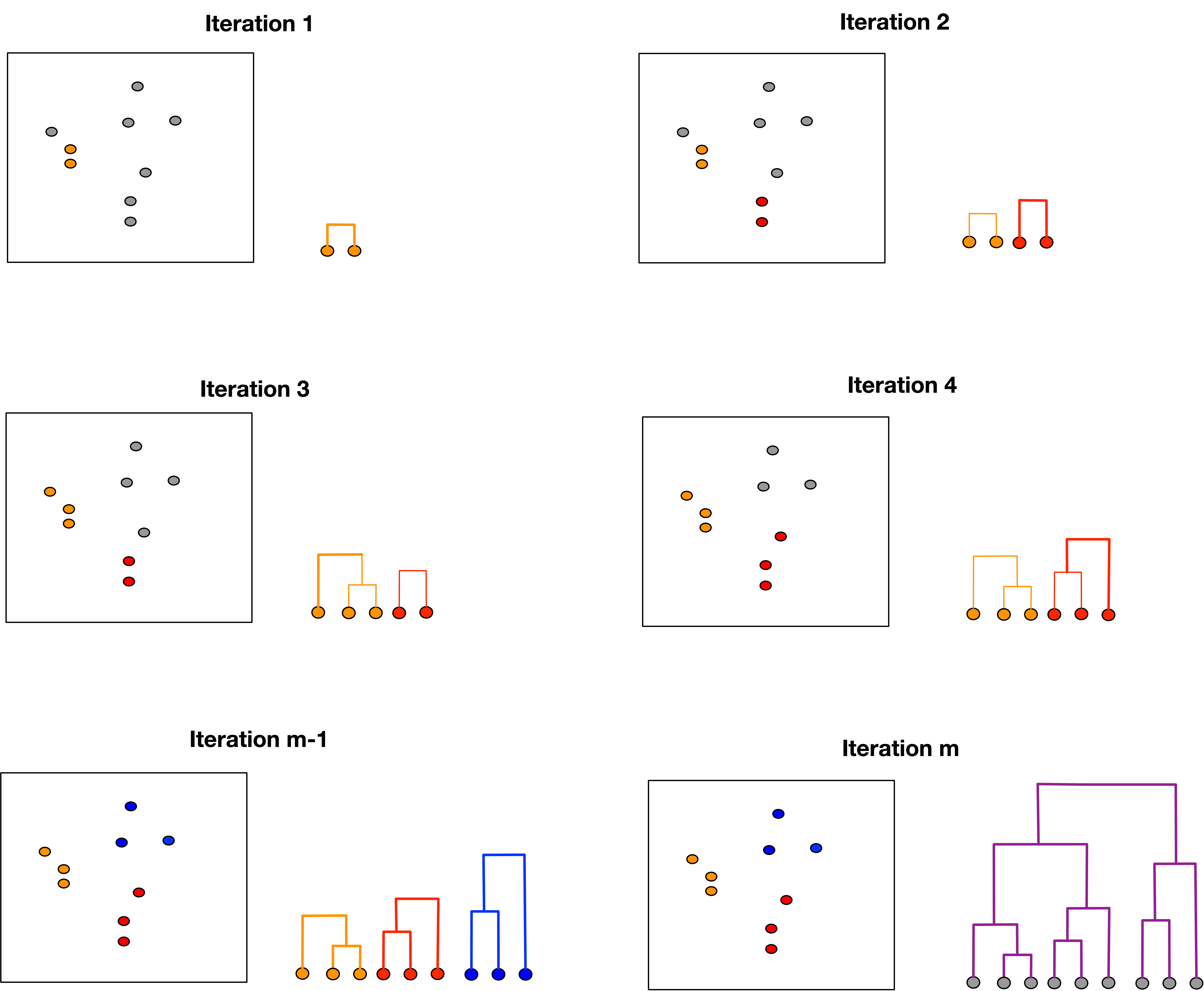
To determine the number of clusters, cut the dendrogram at a certain height and count the resulting branches.

9.3.2 Linkage Methods

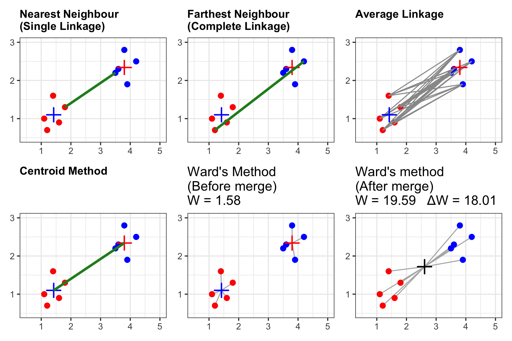
Linkage determines the dissimilarity d(C_1, C_2) between two clusters, C_1 and C_2. The key R function for hierarchical clustering is hclust in the stats package.

Linkage Method	Formula	Description
Single Linkage (Nearest-Neighbor)	d(C_{1},C_{2})=\min_{i\in C_{1},j\in C_{2}}d_{ij}	Distance between closest points in the clusters.
Complete Linkage (Furthest-Neighbor)	d(C_{1},C_{2})=\max_{i\in C_{1},j\in C_{2}}d_{ij}	Distance between farthest points in the clusters.
Average Linkage	d(C_{1},C_{2})=\frac{1}{\|C_{1}\|\cdot\|C_{2}\|}\sum_{i\in C_{1},j\in C_{2}}d_{ij}	Average of all pairwise distances.
Centroid Method	d(\overline{\mathbf{x}}_{A},\overline{\mathbf{x}}_{B})=\bigl\\|\overline{\mathbf{x}}_{A}-\overline{\mathbf{x}}_{B}\bigr\\|^2_2	Distance between centroids (means) of two clusters.
Ward’s Method	\Delta_{SST} = \frac{n_{A}n_{B}}{n_{A}+n_{B}}\bigl\\|\overline{\mathbf{x}}_{A}-\overline{\mathbf{x}}_{B}\bigr\\|^2_2	Merges two clusters that result in the smallest increase in the total within-cluster sum of squared Euclidean distances (SST).

9.3.3 Insect Community Data Example

Insect Community Data

The data set (newpbi.csv) consist of insect counts collected on 30 Iowa prairies with 44 types of insects. Counts of these insects were taken periodically over one summer at the 30 sites. The first column (Site) identifies the sample location, and the second column (Type) is likely a categorical environmental or habitat variable. The remaining columns are abundance counts for different arthropod groups (e.g., Araneae, ACari).

R Code: Load Data

df = read.csv("newpbi.csv")
head(df)

Research Questions

Community Structure
- Question 1: Do distinct communities exist in the sampled areas, and if so, how many? This can discover if the sites fall into natural groupings based purely on the species/taxa they contain. This could reveal previously unrecognized ecological zones or biotypes
- Question 2: Are the natural community clusters consistent with the recorded habitat types (Type)?
Taxonomic and Functional Groups
- Question 3: Which specific arthropod taxa (e.g., specific beetle or fly families) tend to co-occur across sites?

R Code: Visualize the data

abundance_matrix = as.matrix(df[,-c(1:2)])

heatmap(abundance_matrix, col=cm.colors(256), 
               Rowv=NA, Colv=NA)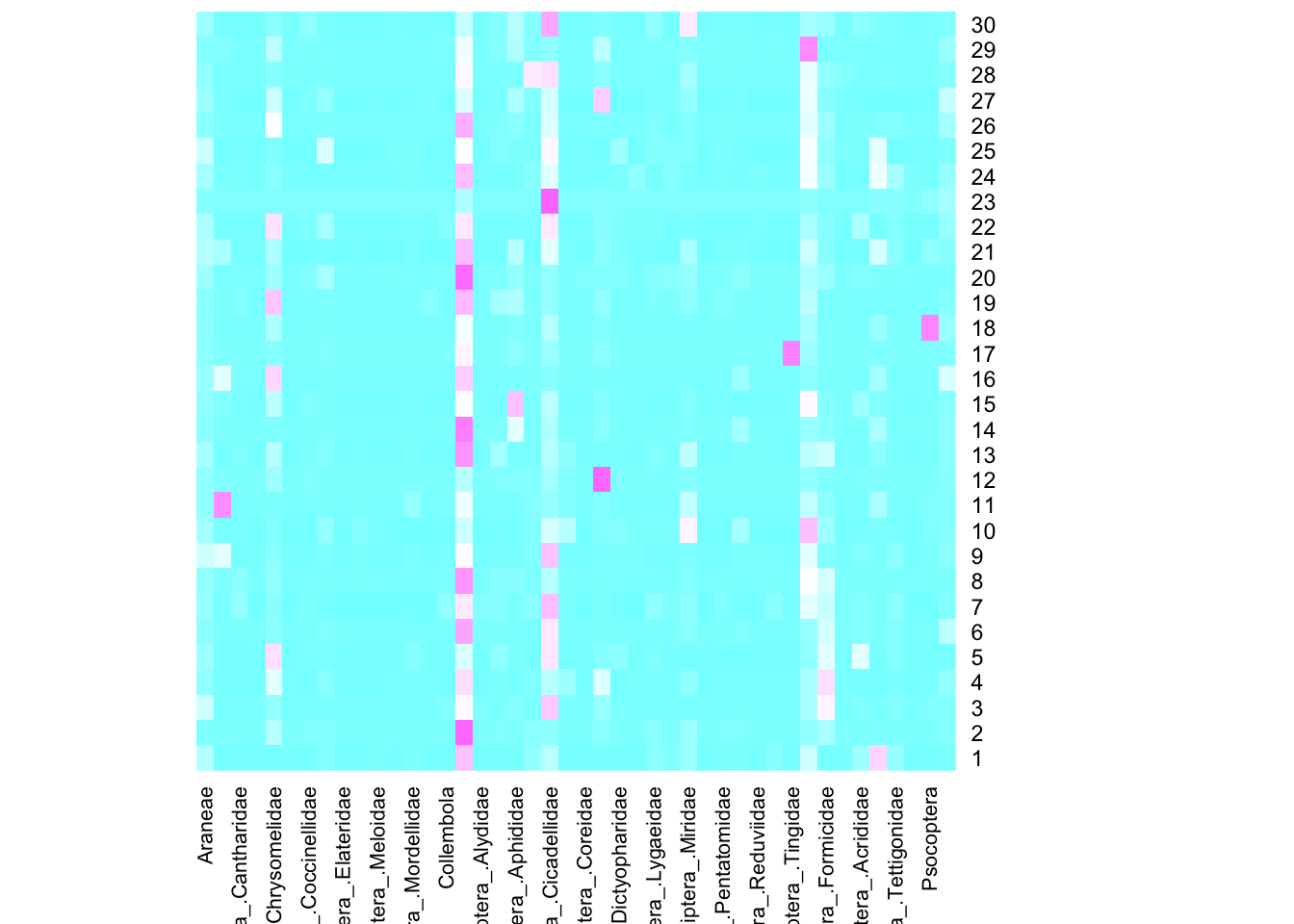

A heatmap displays:
- Observations (or variables) on rows.
- Variables (or observations) on columns.
- Color intensity = value size.

heatmap

heatmap(x, Rowv = NULL, Colv = if(symm)"Rowv" else NULL,
        distfun = dist, hclustfun = hclust,
        reorderfun = function(d, w) reorder(d, w),
        add.expr, symm = FALSE, revC = identical(Colv, "Rowv"),
        scale = c("row", "column", "none"), na.rm = TRUE,
        margins = c(5, 5), ColSideColors, RowSideColors,
        cexRow = 0.2 + 1/log10(nr), cexCol = 0.2 + 1/log10(nc),
        labRow = NULL, labCol = NULL, main = NULL,
        xlab = NULL, ylab = NULL,
        keep.dendro = FALSE, verbose = getOption("verbose"), ...)

By default, heatmap performs clustering for both rows and columns based on the clustering function hclust. Unless we know the default clustering uses an appropriate distance/dissimilarity metric, we can use the clustered heatmap for interpretation.

R Code: Calculate Bray-Curtis dissimilarity via vegdist

library(vegan)
D = vegdist(abundance_matrix, method = "bray")

R Code: Hierarchical Clustering via hclust

hca1 = hclust(D, method="single")
hca2 = hclust(D, method="complete")
hca3 = hclust(D, method="average")
hca4 = hclust(D, method="ward.D2")

R Code: Dendrograms

library(factoextra)
p1=fviz_dend(hca1)
p2=fviz_dend(hca2)
p3=fviz_dend(hca3)
p4=fviz_dend(hca4)

patchwork::wrap_plots(p1 + ggtitle("single"),
                      p2 + ggtitle("complete"),
                      p3 + ggtitle("average"),
                      p4 + ggtitle("ward"),ncol=2)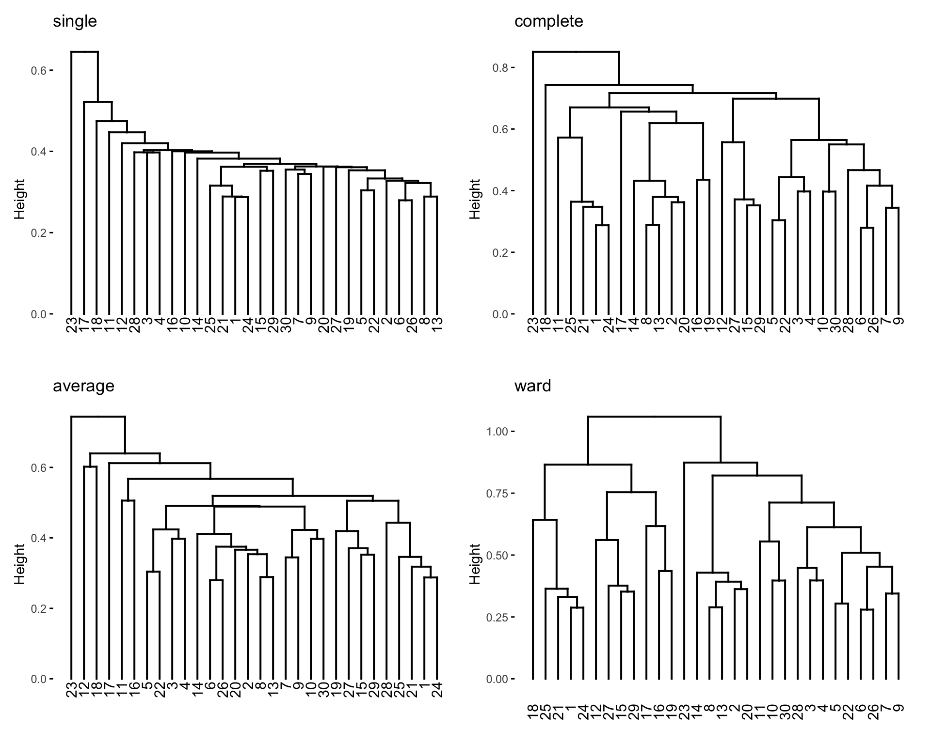

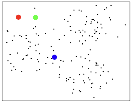
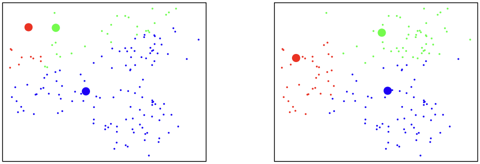
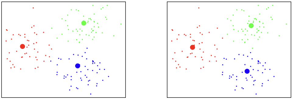
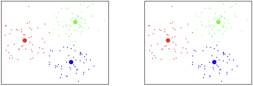
Interpretation: The height at which two branches join represents the dissimilarity (Bray-Curtis distance) between them. Short branches that merge low down indicate highly similar communities.

9.4 K-Means Clustering

K-means clustering is a type non-hierarchical clustering algorithm
No tree structure exists
One often needs to pre-determine the number of clusters in the algorithm to find the clusters

9.4.1 Basic Idea

A K-means clustering algorithm

Initialize: Pick K points randomly as cluster centers.
Repeat:
- Assign points to closet cluster center
- Update cluster center location to the mean of the assigned points
Stop when no points change cluster assignment (convergence)

Illustration of K-means clustering

Iteration 1

Iteration 2

Iteration 3

9.4.2 A Toy Example

This small data set has only four cases (A, B, C, and D) and two variables are measured on each case. The data vectors are: A=\begin{pmatrix}5\\ 3\end{pmatrix} \quad B=\begin{pmatrix}-1\\ 1\end{pmatrix} \quad C=\begin{pmatrix}1\\ -2\end{pmatrix} \quad D=\begin{pmatrix}-3\\ -2\end{pmatrix}

Start with initial clusters \mathbf{(A, B)} and \mathbf{(C, D)}. The centroids for the initial clusters are C_{1}=\begin{pmatrix}2\\ 2\end{pmatrix} \quad \text{and} \quad C_{2}=\begin{pmatrix}-1\\ -2\end{pmatrix}

Step-by-step K-means iteration

In each iteration, we need to compute the distance of each case from each centroid. Here we use Euclidean distance. Then we update cluster centroids.

Iteration 1

distances:
- Case A: d(A,C_{1})=\sqrt{(5-2)^{2}+(3-2)^{2}}=\sqrt{10}, and d(A,C_{2})=\sqrt{(5-(-1))^{2}+(3-(-2))^{2}}=\sqrt{61}
- Case B: d(B,C_{1})=\sqrt{(-1-2)^{2}+(1-2)^{2}}=\sqrt{10}, and d(B,C_{2})=\sqrt{(-1-(-1))^{2}+(1-(-2))^{2}}=\sqrt{9}
- Case C: d(C,C_{1})=\sqrt{(1-2)^{2}+(-2-2)^{2}}=\sqrt{17}, and d(C,C_{2})=\sqrt{(1-(-1))^{2}+(-2-(-2))^{2}}=\sqrt{4}
- Case D: d(D,C_{1})=\sqrt{(-3-2)^{2}+(-2-2)^{2}}=\sqrt{41}, and d(D,C_{2})=\sqrt{(-3-(-1))^{2}+(-2-(-2))^{2}}=\sqrt{4}
The new clusters are \mathbf{(A)} and \mathbf{(B, C, D)}
- The new centroids are: C_{1}=\begin{pmatrix}5\\ 3\end{pmatrix} \quad \text{and} \quad C_{2}=\begin{pmatrix}-1\\ -1\end{pmatrix}
Check convergence: for example, specify a tolerance for the difference between two consecutive centroids.

Iteration 2

Distances:
- Case A: d(A,C_{1})=\sqrt{(5-5)^{2}+(3-3)^{2}}=\sqrt{0} and d(A,C_{2})=\sqrt{(5-(-1))^{2}+(3-(-1))^{2}}=\sqrt{52}
- Case B: d(B,C_{1})=\sqrt{(-1-5)^{2}+(1-3)^{2}}=\sqrt{40} and d(B,C_{2})=\sqrt{(-1-(-1))^{2}+(1-(-1))^{2}}=\sqrt{4}
- Case C: d(C,C_{1})=\sqrt{(1-5)^{2}+(-2-3)^{2}}=\sqrt{41} and d(C,C_{2})=\sqrt{(1-(-1))^{2}+(-2-(-1))^{2}}=\sqrt{5}
- Case D: d(D,C_{1})=\sqrt{(-3-5)^{2}+(-2-3)^{2}}=\sqrt{89} and d(D,C_{2})=\sqrt{(-3-(-1))^{2}+(-2-(-1))^{2}}=\sqrt{5}
- The new clusters are \mathbf{(A)} and \mathbf{(B, C, D)} and the clusters did not change: C_{1}=\begin{pmatrix}5\\ 3\end{pmatrix} \quad \text{and} \quad C_{2}=\begin{pmatrix}-1\\ -1\end{pmatrix}
Stop: The K-means algorithm has converged to produce clusters \mathbf{(A)} and \mathbf{(B, C, D)}

9.4.3 How to Choose the Number of Clusters?

Review of notations

n is the number of observations in the data.
p is the number of variables measured on each observation.
C_k represents the k-th cluster at a particular step of the clustering algorithm and n_k is the number of observations in C_k.
SS_{T} is the total sum of squared distances from the overall vector of means for all n observations in the data set: SS_T = \sum_{i=1}^n (\mathbf{x}_i-\bar{\mathbf{x}})^{\prime} (\mathbf{x}_i-\bar{\mathbf{x}})

Cluster validation metrics

We define the components used in cluster validation metrics:

{G}: The number of groups or clusters. The goal of these methods is to find the optimal {G}.
\mathbf{w}_k: The sum of squared distances for all points within a single cluster, C_k. \mathbf{w}_k:= \sum_{i \text{ in } C_k} (\mathbf{x}_i-\bar{\mathbf{x}}_k)^{\prime} (\mathbf{x}_i-\bar{\mathbf{x}}_k)
\mathbf{W}_G: The total sum of squared distances across all \mathbf{G} clusters. This is the Within-Group Sum of Squares (WCSS): \mathbf{W}_G = \sum_{k=1}^{G} \mathbf{w_k}
\mathbf{B}_G: The Between-Group Sum of Squares (BCSS), which measures the separation of the group centroids. It is defined based on the Total Sum of Squares ({SS}_T): \mathbf{B}_G = {SS}_T - \mathbf{W}_G

Comparative methods

Method	Core Concept	Optimal {G} Rule	Mathematical Metric
Elbow (WCSS)	Measures total compactness (\mathbf{W}_G) as {G} increases.	Choose the {G} where the decrease in \mathbf{W}_G starts to slow significantly (the “bend”).	Plot \mathbf{W}_G vs. {G}
Calinski-Harabasz Index	Maximizes the ratio of separation (\mathbf{B}_G) to compactness (\mathbf{W}_G).	Choose the {G} that maximizes the CH index (highest peak).	\text{CH}(G) = \frac{\mathbf{B}_G}{\mathbf{W}_G} \cdot \frac{n-G}{G-1}
Gap Statistic	Compares the observed compactness (\mathbf{W}_G) to the expected compactness (\mathbf{W}_{G}^) under a random null distribution*.	Choose the smallest {G} that maximizes the Gap statistic.	\text{Gap}(G) = E_{n} \{\log(\mathbf{W}_{G}^*)\} - \log({\mathbf{W}_G})

Note: \mathbf{W}_G^* is defined slightly different from \mathbf{W}_G.

Define D_k = \sum_{i, i'\in C_k} d_{ii'} to be the sum of pairwise distances for all points in cluster C_k.
Set W_G^*=\sum_{k=1}^G \frac{1}{2n_k} D_k.

9.4.4 Working Example

USArests data

library(factoextra)
library(cluster)
#load data
df <- USArrests

#remove rows with missing values
df <- na.omit(df)

df <- scale(df)

head(df)

               Murder   Assault   UrbanPop         Rape
Alabama    1.24256408 0.7828393 -0.5209066 -0.003416473
Alaska     0.50786248 1.1068225 -1.2117642  2.484202941
Arizona    0.07163341 1.4788032  0.9989801  1.042878388
Arkansas   0.23234938 0.2308680 -1.0735927 -0.184916602
California 0.27826823 1.2628144  1.7589234  2.067820292
Colorado   0.02571456 0.3988593  0.8608085  1.864967207

Elbow method

fviz_nbclust(df, kmeans, method = "wss")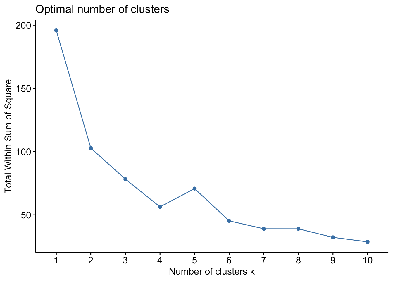

Gap statistic

fviz_nbclust(df, kmeans, method = "gap_stat")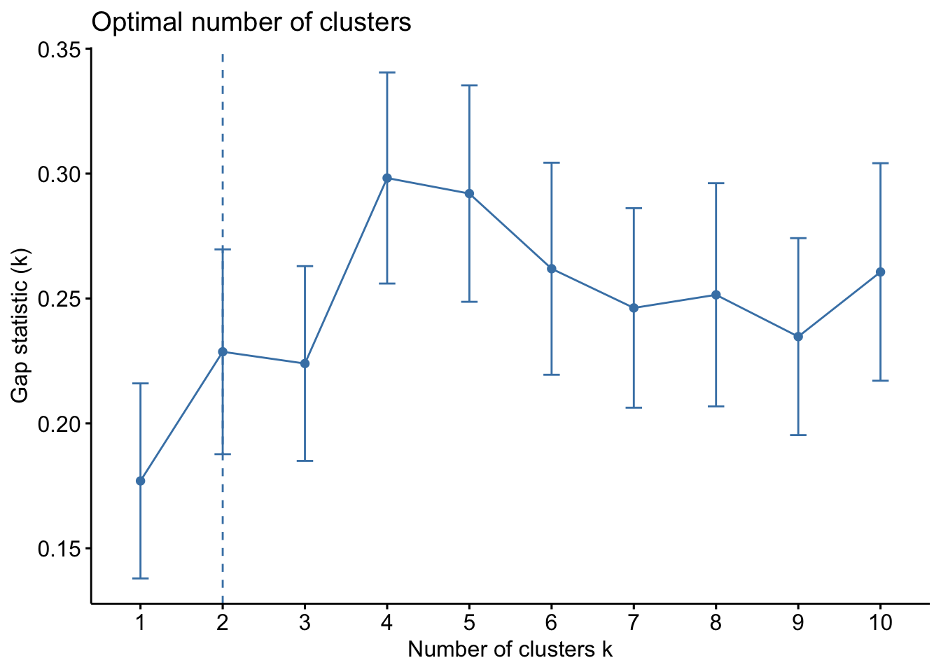

K-means clustering

set.seed(4750)

#perform k-means clustering with k = 4 clusters
km = kmeans(df, 
     centers = 4, 
     nstart = 25 # choose 25 initial centers
     )

print(km)

K-means clustering with 4 clusters of sizes 13, 13, 16, 8

Cluster means:
      Murder    Assault   UrbanPop        Rape
1  0.6950701  1.0394414  0.7226370  1.27693964
2 -0.9615407 -1.1066010 -0.9301069 -0.96676331
3 -0.4894375 -0.3826001  0.5758298 -0.26165379
4  1.4118898  0.8743346 -0.8145211  0.01927104

Clustering vector:
       Alabama         Alaska        Arizona       Arkansas     California 
             4              1              1              4              1 
      Colorado    Connecticut       Delaware        Florida        Georgia 
             1              3              3              1              4 
        Hawaii          Idaho       Illinois        Indiana           Iowa 
             3              2              1              3              2 
        Kansas       Kentucky      Louisiana          Maine       Maryland 
             3              2              4              2              1 
 Massachusetts       Michigan      Minnesota    Mississippi       Missouri 
             3              1              2              4              1 
       Montana       Nebraska         Nevada  New Hampshire     New Jersey 
             2              2              1              2              3 
    New Mexico       New York North Carolina   North Dakota           Ohio 
             1              1              4              2              3 
      Oklahoma         Oregon   Pennsylvania   Rhode Island South Carolina 
             3              3              3              3              4 
  South Dakota      Tennessee          Texas           Utah        Vermont 
             2              4              1              3              2 
      Virginia     Washington  West Virginia      Wisconsin        Wyoming 
             3              3              2              2              3 

Within cluster sum of squares by cluster:
[1] 19.922437 11.952463 16.212213  8.316061
 (between_SS / total_SS =  71.2 %)

Available components:

[1] "cluster"      "centers"      "totss"        "withinss"     "tot.withinss"
[6] "betweenss"    "size"         "iter"         "ifault"

Visualiazing clusters

fviz_cluster(km, data = df)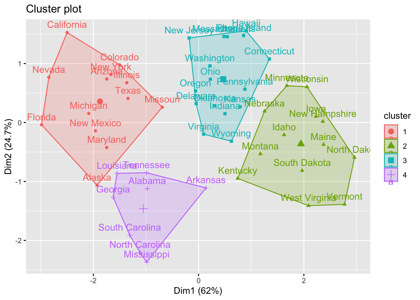

Compute cluster means

aggregate(USArrests, by=list(cluster=km$cluster), mean)

Code

#add cluster assigment to original data
final_data = cbind(USArrests, cluster = km$cluster)

#view final data
head(final_data)