3  Multivariate Normal Distribution

3.1 Why Multivariate Normal?

The univariate normal distribution is fundamental in statistics. But real data usually involve multiple variables measured on the same subjects, and these are often correlated.

• Height and weight of students, or exam scores in different subjects.

Recall that if a random variable X has a normal distribution with mean \mu and variance \sigma^2, its density function has the form f(x) = \frac{1}{ \sqrt{2 \pi } \sigma} \exp \left\{-\frac{1}{2\sigma^2} (x - \mu)^2 \right\}, \;\;\;\; -\infty < x < \infty.

3.2 Matrix Background

• The inverse of a p\times p matrix A is denoted by A^{-1}.
• if A^{-1} exists, A^{-1} is the unique matrix such that AA^{-1} = A^{-1}A = I = \left[ \begin{array}{ccccc} 1 & 0 & \cdots & 0 & 0 \\ 0 & 1 & \cdots & 0 & 0 \\ \vdots & \vdots & \ddots & \vdots & \vdots \\ 0 & 0 & \cdots & 1 & 0 \\ 0 & 0 & \cdots & 0 & 1 \end{array} \right]
  
• A is said to be symmetric if A is the same as its transpose, i.e., A=A^\top or A = A'.
• A is said to be positive definite if \left[ \begin{array}{cccc} x_1 & x_2 & \cdots & x_p \end{array} \right] A \left[ \begin{array}{c} x_1 \\ x_2 \\ \vdots \\ x_p \end{array} \right] > 0 \quad \text{for any} \quad \left[ \begin{array}{cccc} x_1 & x_2 & \cdots & x_p \end{array} \right] \neq \mathbf{0}
• If A is positive definite, then A^{-1} exists.

Exercise: Matrix Algebra

A = matrix(c(2,1,1,4), ncol=2, byrow=TRUE)
A

     [,1] [,2]
[1,]    2    1
[2,]    1    4

a = 2 
a * A

     [,1] [,2]
[1,]    4    2
[2,]    2    8

B = matrix(c(1,2,2,9), ncol=2, byrow=TRUE)
A + B 

     [,1] [,2]
[1,]    3    3
[2,]    3   13

x = c(1,2)
A %*% x 

     [,1]
[1,]    4
[2,]    9

A %*% B 

     [,1] [,2]
[1,]    4   13
[2,]    9   38

# matrix inversion
solve(A)

           [,1]       [,2]
[1,]  0.5714286 -0.1428571
[2,] -0.1428571  0.2857143

# check result
A %*% solve(A)

     [,1] [,2]
[1,]    1    0
[2,]    0    1

3.2.1 Eigenvalues and Eigenvectors

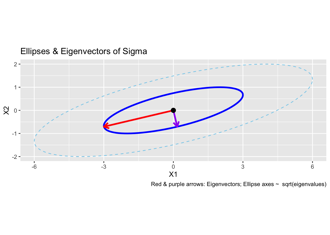
Definition

Given a p \times p square matrix A, an eigenvector \mathbf{v} and its corresponding eigenvalue \lambda satisfy: A \mathbf{v} = \lambda \mathbf{v}

Interpretation: Multiplying A by its eigenvector \mathbf{v} simply stretches or shrinks \mathbf{v} by a factor \lambda—the direction of \mathbf{v} does not change.

• Why Do They Matter?

  • Eigenvectors show the principal directions in which A stretches or compresses the space.
  • In statistics, the eigenvectors of a covariance matrix gives the directions of maximum variance.
  • The corresponding eigenvalues tell you how much variance there is in each direction as explained below.

• Some Properties

  • If (\lambda_j, \mathbf{e}_j) is an eigenvalue-eigenvector pair for a p \times p matrix A, by definition A \mathbf{e}_j = \lambda_j \mathbf{e}_j.
  • Eigenvectors are usually scaled to have length one, i.e., 1=\mathbf{e}_j^{\top} \mathbf{e}_j = e_{j1}^2+e_{j2}^2 + \cdots + e_{jp}^2.
  • Eigenvectors are mutually orthogonal, i.e., \mathbf{e}_j^{\top} \mathbf{e}_k = 0 for any j \ne k.
  • (\lambda_j^{-1}, \mathbf{e}_j) is an eigenvalue-eigenvector pair of A^{-1} when A is positive definite and A^{-1} exists.

3.2.2 Spectral Decomposition

Spectral decomposition

For any p\times p symmetric matrix A, its spectral decomposition is A = \lambda_1 \mathbf{e}_1 \mathbf{e}_1^{\top} + \lambda_2 \mathbf{e}_2 \mathbf{e}_2^{\top} + \cdots + \lambda_p \mathbf{e}_p \mathbf{e}_p^{\top}

• If A^{-1} exists, then A^{-1} = \lambda_1^{-1} \mathbf{e}_1 \mathbf{e}_1^{\top} + \lambda_2^{-1} \mathbf{e}_2 \mathbf{e}_2^{\top} + \cdots + \lambda_p^{-1} \mathbf{e}_p \mathbf{e}_p^{\top}.
• A^{1/2} = \lambda_1^{1/2} \mathbf{e}_1 \mathbf{e}_1^{\top} + \lambda_2^{1/2} \mathbf{e}_2 \mathbf{e}_2^{\top} + \cdots + \lambda_p^{1/2} \mathbf{e}_p \mathbf{e}_p^{\top}
• A^{-1/2} = \lambda_1^{-1/2} \mathbf{e}_1 \mathbf{e}_1^{\top} + \lambda_2^{-1/2} \mathbf{e}_2 \mathbf{e}_2^{\top} + \cdots + \lambda_p^{-1/2} \mathbf{e}_p \mathbf{e}_p^{\top}
• A^{1/2} A^{1/2} = A and A^{-1/2}A^{-1/2}=A^{-1}.

A = matrix(c(4, 2, 1, 3), nrow = 2)

eig = eigen(A)
print(eig)

eigen() decomposition
$values
[1] 5 2

$vectors
          [,1]       [,2]
[1,] 0.7071068 -0.4472136
[2,] 0.7071068  0.8944272

3.2.3 Determinant of a p\times p matrix

• The determinant of the matrix A is denoted by |A| or \text{det}(A).
• The determinant of a p \times p matrix is the product of its eigenvalues, i.e., |A| = \text{det}(A) = \lambda_1 \lambda_2 \cdots \lambda_p.
• All of the eigenvalues of a positive definite matrix are positive.
• The determinant of a positive definite matrix must be larger than zero.
• If at least one eigenvalue is zero and the inverse of the matrix does not exist, then the determinant of the matrix is zero.

det(A) 

[1] 10

E = eigen(A)
prod(E$values)

[1] 10

3.3 Probability Density Function of MVN

The multivariate normal distribution (MVN) generalizes the univariate normal distribution to multiple variables.

A random vector \mathbf{x} = (x_1, x_2, \ldots, x_p)^\top follows a multivariate normal distribution if every linear combination of its components is normal. We use the notation: \mathbf{x} \sim N_p(\boldsymbol{\mu}, {\Sigma}) \quad \text{ or }\quad \mathbf{x} \sim \text{MVN}(\boldsymbol\mu, \Sigma) where

• \boldsymbol{\mu}:=(\mu_1, \mu_2, \ldots, \mu_p)^\top is the p-dimensional mean vector
• and \Sigma = \left[ \begin{array}{cccc} \sigma_{11} & \sigma_{12} & \cdots & \sigma_{1p} \\ \sigma_{21} & \sigma_{22} & \cdots \ & \sigma_{2p} \\ \vdots & \vdots & \ddots & \vdots \\ \sigma_{p1} & \sigma_{p2} & \cdots & \sigma_{pp} \end{array} \right] is the p \times p covariance matrix of \mathbf{x}.

Probability Density Function (PDF)

The probability density function for \mathbf{x} \sim N_p(\boldsymbol \mu, \Sigma) is f(\mathbf{x}) = (2\pi)^{-p/2} |\Sigma|^{-1/2} \exp\left(-\frac{1}{2}(\mathbf{x}-\boldsymbol\mu)^\top \Sigma^{-1}(\mathbf{x}-\boldsymbol\mu)\right)

Geometric Interpretation:

• \boldsymbol{\mu}: The center of the point cloud.
• {\Sigma}: Controls the spread and orientation.
  • Diagonal = variances
  • Off-diagonal = covariances (correlation/shape)

Mahalanobis Distance

The quadratic form (\mathbf{x}-\boldsymbol\mu)^\top \Sigma^{-1}(\mathbf{x}-\boldsymbol\mu) in the density formula is the squared statistical distance of \mathbf{x} from \boldsymbol\mu. It is often referred to as the square of the Mahalanobis distance.

3.3.1 Some Properties

If \mathbf{x} \sim N_p(\boldsymbol\mu, \Sigma), then the following statements are true:

1. Marginal distributions: Each variable is normally distributed, i.e., x_i \sim N(\mu_i, \sigma_{ii}).
2. Any linear combinations is normal: Let a_1, \ldots, a_p \in \mathbb{R}. Then \mathbf{a}^\top \mathbf{x} = \sum_{i=1}^p a_i x_i \sim N(\mathbf{a}^\top \boldsymbol \mu, \mathbf{a}^\top \Sigma \mathbf{a})
3. If \mathbf{x} \sim N_p(\boldsymbol \mu, \Sigma), then (\mathbf{x}-\boldsymbol\mu)^\top \Sigma^{-1}(\mathbf{x}-\boldsymbol\mu) \sim \chi_p^2
4. Conditional distributions: Any subset of variables, conditional on others, is normal.
5. Elliptical contours: The joint density forms ellipses.

3.3.2 R Exercise: MVN Properties

mu = c(0,0)
Sigma = matrix(c(2,1,1,4),ncol=2, byrow=TRUE)
a = c(1,1)

# simulate from MVN
set.seed(4750)
x = MASS::mvrnorm(1, mu=mu, Sigma=Sigma)

# linear combination  
t(a) %*% x 

           [,1]
[1,] -0.4976936

# quadratic form 
t(x-mu)%*%solve(Sigma)%*%(x-mu)

           [,1]
[1,] 0.07250492

3.4 Visualizing the MVN in R

3.4.1 Visualizing Marginal Distributions

library(MASS) 
set.seed(4750) 
mu <- c(0, 0) 
Sigma_none <- matrix(c(1, 0, 0, 1), nrow=2) 
Sigma_pos <- matrix(c(1, 0.8, 0.8, 1), nrow=2) 
Sigma_neg <- matrix(c(1, -0.8, -0.8, 1), nrow=2)

X_none <- mvrnorm(500, mu, Sigma_none) 
X_pos <- mvrnorm(500, mu, Sigma_pos) 
X_neg <- mvrnorm(500, mu, Sigma_neg)

par(mfrow = c(1,3)) 
plot(X_none, main="No Correlation", xlab="X1", ylab="X2", col=rgb(0,0,1,0.3), pch=16) 
plot(X_pos, main="Positive Correlation", xlab="X1", ylab="X2", col=rgb(0,0.5,0,0.3), pch=16) 
plot(X_neg, main="Negative Correlation", xlab="X1", ylab="X2", col=rgb(1,0,0,0.3), pch=16)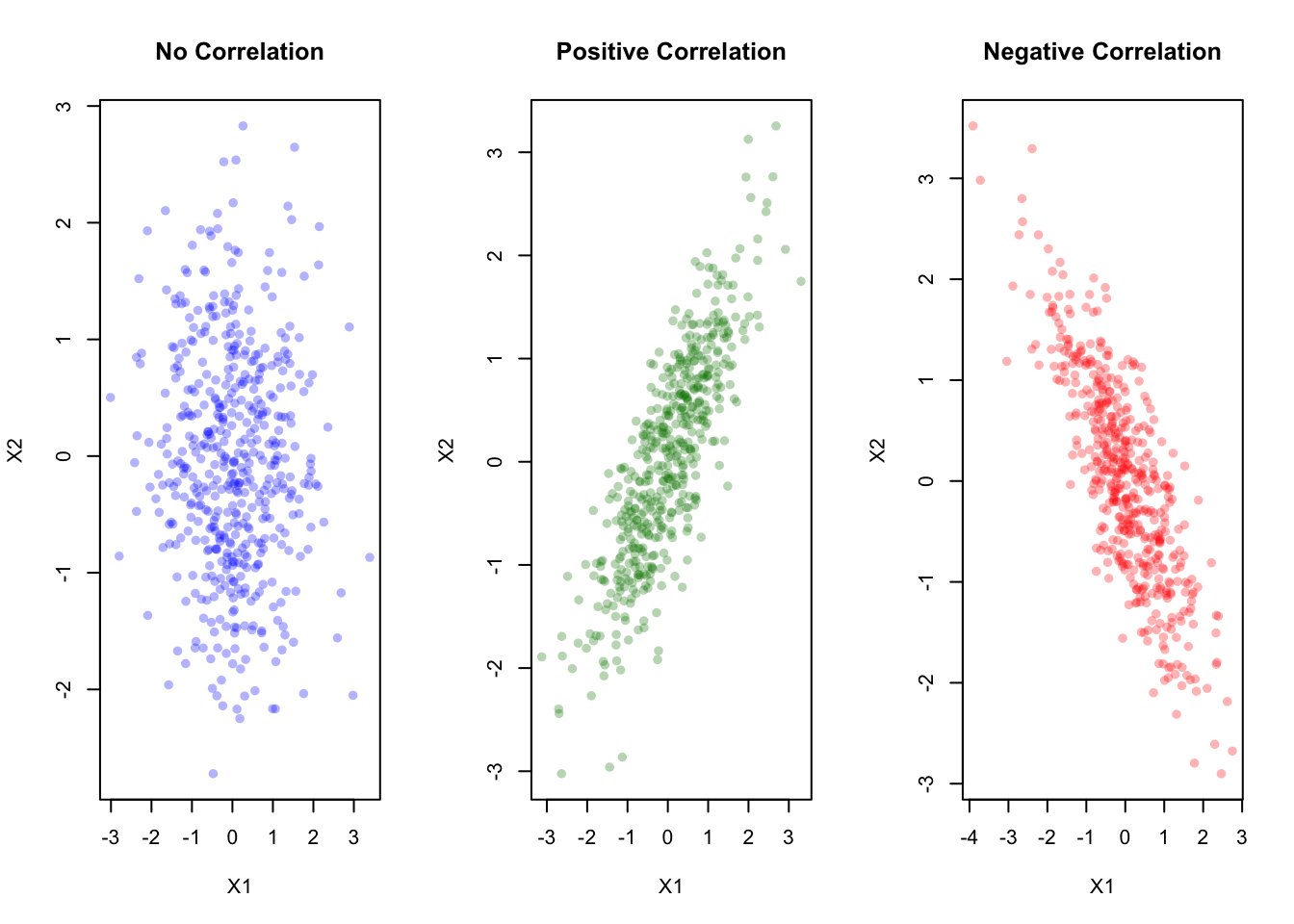 

Exercise

Try changing the covariance matrix \Sigma in the code above.

• What happens if you set the off-diagonal entries to 0?
• What about +0.9 or -0.9?

View Solution

Let’s visualize how changing the off-diagonal entries (correlation) in \Sigma affects the bivariate normal:

library(MASS)
set.seed(4750)
mu <- c(0, 0)

# Case 1: No correlation (off-diagonal = 0)
Sigma_none <- matrix(c(1, 0, 0, 1), nrow=2)
X_none <- mvrnorm(500, mu, Sigma_none)

# Case 2: Strong positive correlation (off-diagonal = +0.9)
Sigma_pos <- matrix(c(1, 0.9, 0.9, 1), nrow=2)
X_pos <- mvrnorm(500, mu, Sigma_pos)

# Case 3: Strong negative correlation (off-diagonal = -0.9)
Sigma_neg <- matrix(c(1, -0.9, -0.9, 1), nrow=2)
X_neg <- mvrnorm(500, mu, Sigma_neg)

par(mfrow = c(1,3))
plot(X_none, main = "No correlation", xlab = "X1", 
     ylab = "X2", col = rgb(0,0,1,0.4), pch = 16)
plot(X_pos, main = "Positive correlation", xlab = "X1",
     ylab = "X2", col = rgb(0,0.5,0,0.4), pch = 16)
plot(X_neg, main = "Negative correlation", xlab = "X1",
     ylab = "X2", col = rgb(1,0,0,0.4), pch = 16)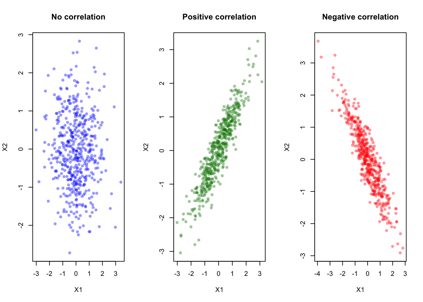

3.4.2 Density Contour

• A set of all vectors \mathbf{x} that correspond to a constant height of the density function forms an ellipsoid centered at \boldsymbol\mu.
• The MVN density is constant for all \mathbf{x}’s that are the same statistical distance from the population mean vector, i.e., all \mathbf{x}’s that satisfy \sqrt{(\mathbf{x}-\boldsymbol\mu)^\top \Sigma^{-1}(\mathbf{x}-\boldsymbol\mu)} = \text{constant}.
• The axes of the ellipses are in the directions of the eigenvectors of \Sigma and the length of the j-th longest axis is proportional to \sqrt{\lambda_{j}}, where \lambda_{j} is the eigenvalue associated with the j-th eigenvector of \Sigma.

Interpretation:

• The ellipse shows a constant-density contour for the MVN.
• The red and purple arrows indicate eigenvectors of \Sigma.
• The lengths of these arrows are proportional to \sqrt{\lambda_j}.

library(mvtnorm)
library(ggplot2)

mu = c(0, 0)
Sigma = matrix(c(1, 0.7, 0.7, 1), 2)

# Create grid
x = seq(-3, 3, length=100)
y = seq(-3, 3, length=100)
grid = expand.grid(x = x, y = y)

# Compute density at each grid point
grid$z = mvtnorm::dmvnorm(as.matrix(grid), 
                           mean = mu, sigma = Sigma)

# Plot contours
ggplot(grid, aes(x = x, y = y, z = z)) +
  geom_contour_filled(bins = 15) +
  coord_fixed() +
  labs(title = "Bivariate Normal Density (Contours)",
       x = "X1", y = "X2", fill = "Density") +
  theme_minimal()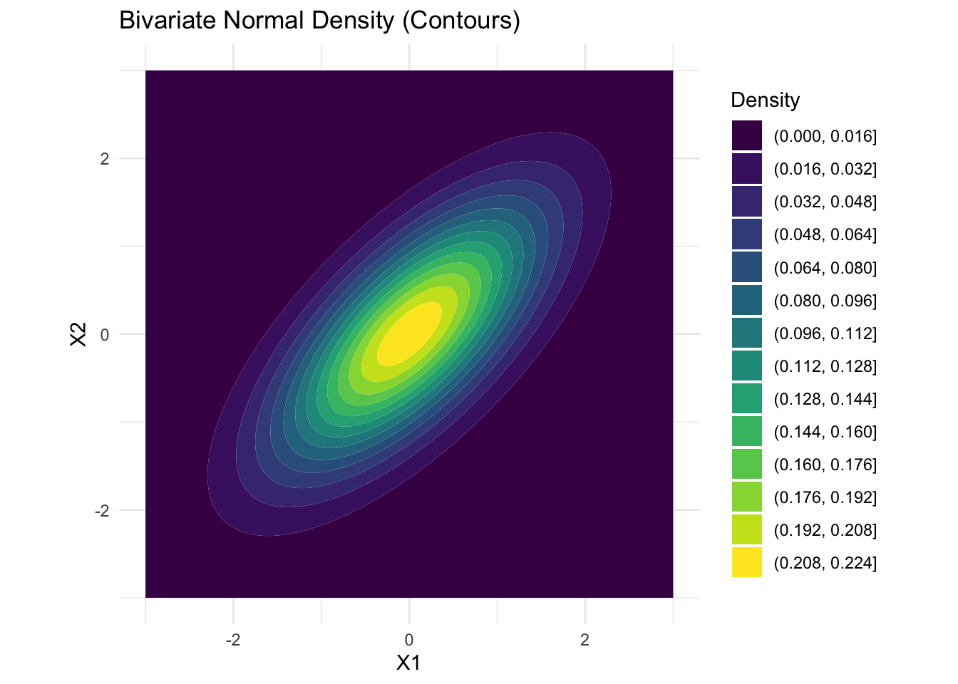

3.4.3 3D Surface Plot

library(plotly)

z_matrix <- matrix(grid$z, nrow = length(x), byrow = FALSE)
plot_ly(x = x, y = y, z = z_matrix) %>%
  add_surface(
    contours = list(
      z = list(show = TRUE, 
               usecolormap = TRUE, 
               highlightcolor = "#ff0000", 
               project = list(z = TRUE)))) %>%
  layout(title = "Bivariate Normal Density (Surface)",
         scene = list(xaxis = list(title = "X1"),
                      yaxis = list(title = "X2"),
                      zaxis = list(title = "Density")))

3.5 Central (1-\alpha)\times 100\% Region of MVN

3.5.1 Properties of Density Contours

Definition

• The probability is 1 - \alpha that the value of a random vector will be inside the ellipsoid defined by (\mathbf{x}-\boldsymbol\mu)^\top \Sigma^{-1}(\mathbf{x}-\boldsymbol\mu) \leq \chi^2_{(p), 1-\alpha} where \chi^2_{(p),1-\alpha} is the upper (100 \times \alpha) percentile of a chi-square distribution with p degrees of freedom.
• This is smallest region that has probability (1-\alpha) of containing a vector of observations randomly selected from the population.
• The jth axis of this ellipsoid is determined by the eigenvector associated with the j-th largest eigenvalue of \Sigma, for j = 1,...,p.
• The distance along the j-th axis from the center to the boundary of the ellipsoid is \sqrt{\lambda_j} \left( \frac{2}{p \Gamma(p/2)} \right)^{1/p} \sqrt{ \chi^2_{(p), 1-\alpha}}

3.5.2 Geometric Properties

• The ratio of the lengths of the major and minor axes is \frac{\text{Length of major axis}}{\text{Length of minor axis}}=\frac{\sqrt{\lambda_1}}{\sqrt{\lambda_2}}
• The area of the ellipse containing the central (1-\alpha) \times 100 \% of a bivariate normal population is area = \pi \chi^2_{(2), 1-\alpha} \sqrt{\lambda_1} \sqrt{\lambda_2} =\pi \chi^2_{(2),1-\alpha} |\Sigma|^{1/2}
• For p-dimensional normal distributions the hypervolume of the p-dimensional ellipsoid is \frac{2\pi^{p/2}}{p \Gamma(p/2)} \left[\chi^2_{(p),1-\alpha}\right]^{p/2} |\Sigma|^{1/2}

Gamma function

• \Gamma(1) is defined to be 1.0,
• \Gamma\left(\frac{p}{2}\right)=\left(\frac{p}{2}-1\right)\left(\frac{p}{2}-2\right) \cdots (2)(1) when p is an even integer,
• and \Gamma(\frac{p}{2})=\frac{(p-2)(p-4) \cdots(3)(1)}{ 2^{(p-1)/2}} \sqrt{\pi} when p is an odd integer

3.5.3 50% and 90% Contours for Two Bivariate Normals

library(MASS)
library(ggplot2)
library(mvtnorm)

# Two bivariate normals: different means, same covariance
mu1 <- c(0, 0)
mu2 <- c(2, 2)
Sigma <- matrix(c(2, 1.2, 1.2, 2), 2)

# Grid for density evaluation
x <- seq(-3, 6, length=120)
y <- seq(-3, 6, length=120)
grid <- expand.grid(x=x, y=y)
xy = as.matrix(grid)
z1 <- dmvnorm(xy, mean=mu1, sigma=Sigma)
z2 <- dmvnorm(xy, mean=mu2, sigma=Sigma)
grid$z1 = z1 
grid$z2 = z2

# Find contour levels for 50% and 90%
get_density_level <- function(mu, Sigma, p) {
  d2 <- qchisq(p, df=2)
  detS <- det(Sigma)
  norm_const <- 1/(2*pi*sqrt(detS))
  exp_part <- exp(-0.5 * d2)
  norm_const * exp_part
}
level_50 <- get_density_level(mu1, Sigma, 0.5)
level_90 <- get_density_level(mu1, Sigma, 0.9)

# Plot
ggplot() +
  geom_contour(data=grid, aes(x=x, y=y, z=z1), 
               breaks=c(level_50, level_90),
               color="blue", size=1.2, linetype="solid") +
  geom_contour(data=grid, aes(x=x, y=y, z=z2), 
               breaks=c(level_50, level_90),
               color="red", size=1.2, linetype="dashed") +
  geom_point(aes(x=mu1[1], y=mu1[2]), color="blue", size=3) +
  geom_point(aes(x=mu2[1], y=mu2[2]), color="red", size=3) +
  annotate("text", x=mu1[1], y=mu1[2]-0.5, 
           label="mu1", color="blue") +
  annotate("text", x=mu2[1], y=mu2[2]+0.5, 
           label="mu2", color="red") +
  coord_fixed() +
  labs(
    title="50% (inner) and 90% (outer) Contours of Two Bivariate Normals",
    x="X1", y="X2", 
    caption="Density peaks at the mean for each distribution.") +
  theme_minimal()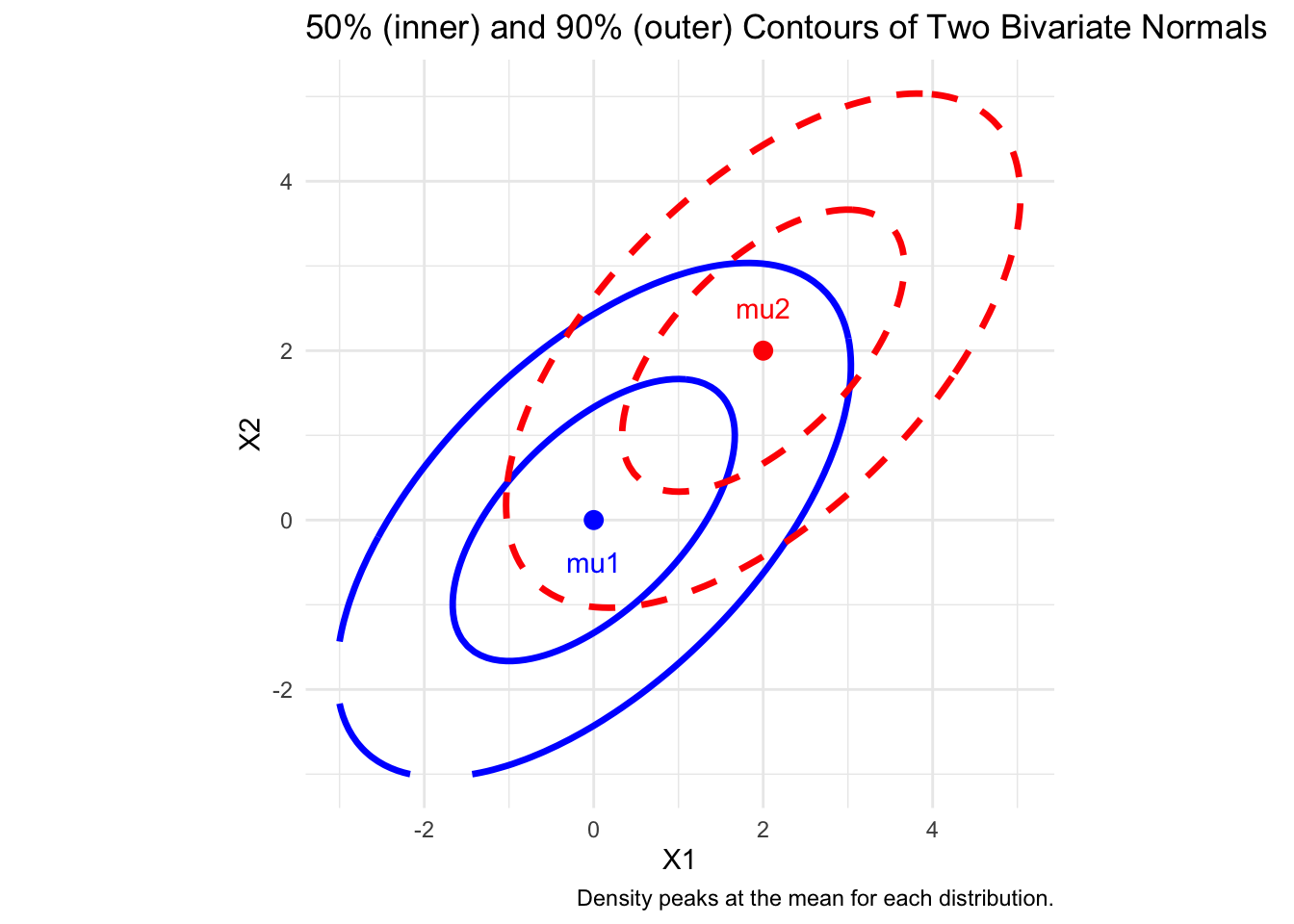

3.6 Overall Measures of Variability

Measures of variability

• Generalized variance and generalized standard deviation tell us about the overall “multivariate” spread or “joint variability”—not just variable by variable, but how “big” the whole data cloud is, including dependencies.
• Total variance tells us the aggregate variance but is “blind” to how variables overlap (i.e., to correlations).

3.6.1 Generalized Variance

• Definition: |\Sigma|=\lambda_1\lambda_2\cdots\lambda_p
• The generalized variance measures the overall spread of the data in all directions at once.
• If any variable has no variation, or if there’s perfect linear dependence (collinearity), the generalized variance drops to zero (the volume “flattens”).

3.6.2 Generalized Standard Deviation

• Definition: |\Sigma|^{1/2}=\sqrt{\lambda_1\lambda_2\cdots\lambda_p}
• The generalized standard deviation is proportional to the volume of the ellipsoid.

3.6.3 Total Variance

• Definition \begin{aligned} trace(\Sigma)\equiv tr(\Sigma)&:= \sigma_{11} + \sigma_{22} + \cdots + \sigma_{pp} \\ &= \lambda_1+\lambda_2+\cdots+\lambda_p \end{aligned}
• This is the total marginal variability in all directions, but does not account for correlation.
• In the ellipsoid analogy, it’s the sum of the squared axis lengths (not the “volume”).

3.6.4 Example: iris Dataset

The iris dataset is a classic and widely used dataset in R, commonly employed for statistical analysis, machine learning, and data visualization. It is built into R and can be loaded directly. Let’s compute the overall measures of the dataset.

# Use iris measurements
X <- iris[, 1:4]
head(X)

  Sepal.Length Sepal.Width Petal.Length Petal.Width
1          5.1         3.5          1.4         0.2
2          4.9         3.0          1.4         0.2
3          4.7         3.2          1.3         0.2
4          4.6         3.1          1.5         0.2
5          5.0         3.6          1.4         0.2
6          5.4         3.9          1.7         0.4

# compute covariance 
S <- cov(X)
print(S)

             Sepal.Length Sepal.Width Petal.Length Petal.Width
Sepal.Length    0.6856935  -0.0424340    1.2743154   0.5162707
Sepal.Width    -0.0424340   0.1899794   -0.3296564  -0.1216394
Petal.Length    1.2743154  -0.3296564    3.1162779   1.2956094
Petal.Width     0.5162707  -0.1216394    1.2956094   0.5810063

eig <- eigen(S)
lambda <- eig$values

# Generalized variance: product of eigenvalues
gen_var <- prod(lambda)
# Generalized standard deviation: sqrt of product
gen_sd <- sqrt(prod(lambda))
# Total variance: sum of eigenvalues
total_var <- sum(lambda)
library(tibble)
result = tibble(
  "Generalized variance" = gen_var,
  "Generalized standard deviation" = gen_sd,
  "Total variance" = total_var
)
print(t(result))

                                     [,1]
Generalized variance           0.00191273
Generalized standard deviation 0.04373476
Total variance                 4.57295705

3.7 Assessing Normality

• Assessing multivariate normality is difficult.
• If any single variable does not have a normal distribution, then the joint distribution of p random variables cannot have a normal distribution.
• We can check normality for each variable individually. If we reject normality for any variable then the joint distribution is not multivariate normal.
• Also look at scatter plots of pairs of variables.
• Look for outliers.

3.7.1 Normal Q-Q plots

• A quantile-quantile (Q-Q) plot can also be constructed for each of the p variables.
• In a Q-Q plot, we plot the ordered data (sample quantiles) against the quantiles that would be expected if the sample came from a standard normal distribution.
• If the hypothesis of normality holds, the points in the plot will fall closely along a straight line.

Normal Q-Q plots

• The slope of the line passing through the points is an estimate of the population standard deviation.
• The intercept of the estimated line is an estimate of the population mean.
• The sample quantiles are just the sample order statistics. For a sample x_1, x_2,...,x_n, quantiles are obtained by ordering sample observations x_{(1)} \leq x_{(2)} \leq ... \leq x_{(n)}, where x_{(j)} is the jth smallest sample observation.

# Normal Q-Q plots for all variables in iris[, 1:4]
par(mfrow = c(2,2))
for (i in 1:4) {
  qqnorm(iris[,i], main = colnames(iris)[i])
  qqline(iris[,i], col = "blue", lwd = 2)
}

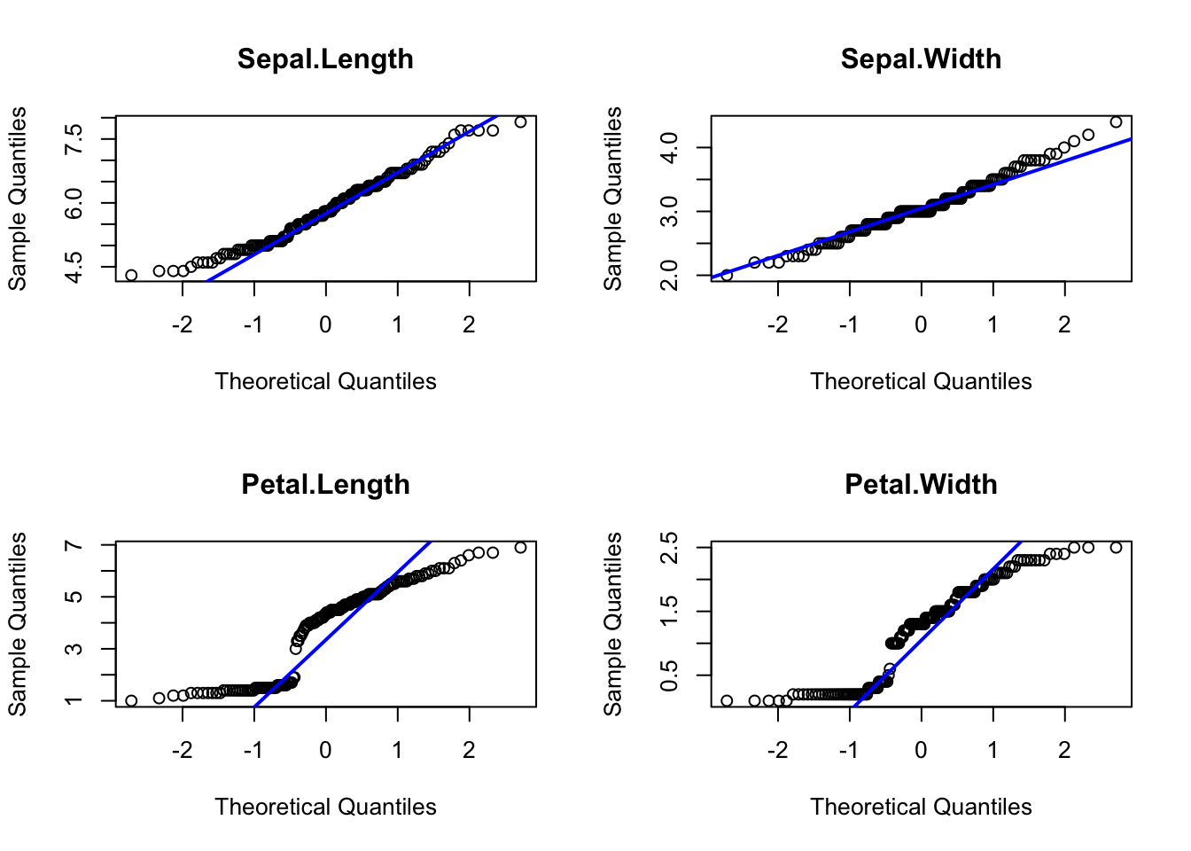
Interpretation:

• If the points follow the line closely, that variable is approximately normal.
• Systematic departures from the line (curves, s-shapes, outliers) suggest non-normality.

# Also look at scatterplots for pairs of variables
pairs(iris[,1:4], main = "Scatterplots: Iris Variables")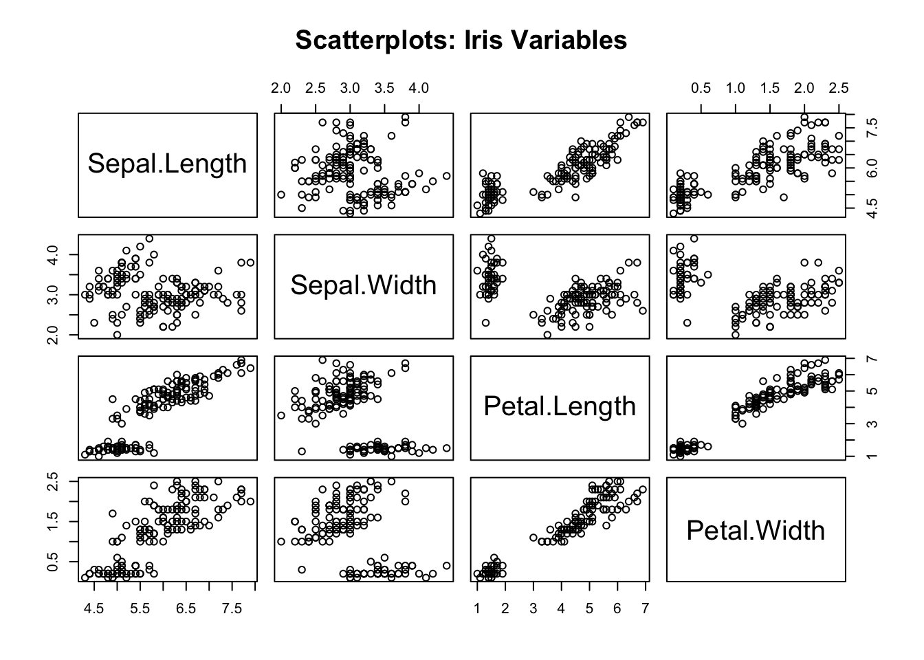

Interpretation: - Outliers, nonlinear patterns, or heavy tails in these scatterplots suggest deviations from the multivariate normal model.

3.7.2 Shapiro-Wilk Test

• The Shapiro-Wilk test is a statistical test for normality. If the p-value is small (typically <0.05), we reject the null hypothesis of normality.

• Test statistic: A weighted correlation between the x_{(j)} and the q_{(j)}: W = \left( \frac{\sum_{i = 1}^n a_j(x_{(i)} - \bar{x})(q_{(i)} - \bar{q}) }{\sqrt{\sum_{i = 1}^n a_j^2(x_{(i)} - \bar{x})^2}\sqrt{\sum_{i = 1}^n (q_{(i)} - \bar{q})^2}} \right)^2.

• We expect values of W to be close to one if the sample arises from a normal population.

• Reject the null hypothesis that data were sampled from a normal distribution if W is too small.

• This test has been extended to p-dimensional normal distributions.

Shapiro-Wilk Test

The Shapiro-Wilk test only checks marginal normality, not joint/multivariate normality when applied to each variable individually. This univariate test is implemented in the R function shapiro.test. To perform multivariate normaltiy check, we need to use the multivariate version of the Shapiro-Wilk test using the function mvShapiro.Test from the package mvShapiroTest.

# Shapiro-Wilk test for each of the four numeric iris variables
apply(iris[, 1:4], 2, shapiro.test)

$Sepal.Length

    Shapiro-Wilk normality test

data:  newX[, i]
W = 0.97609, p-value = 0.01018


$Sepal.Width

    Shapiro-Wilk normality test

data:  newX[, i]
W = 0.98492, p-value = 0.1012


$Petal.Length

    Shapiro-Wilk normality test

data:  newX[, i]
W = 0.87627, p-value = 7.412e-10


$Petal.Width

    Shapiro-Wilk normality test

data:  newX[, i]
W = 0.90183, p-value = 1.68e-08

library(mvShapiroTest)
# multivariate Shapiro-Wilk test 
mvShapiro.Test(as.matrix(iris[, 1:4]))

    Generalized Shapiro-Wilk test for Multivariate Normality by
    Villasenor-Alva and Gonzalez-Estrada

data:  as.matrix(iris[, 1:4])
MVW = 0.97327, p-value = 1.655e-06

Exercise: Assessing Normality with Real Data (mtcars)

Using the mtcars dataset, explore the relationship between mpg (miles per gallon) and hp (horsepower):

1. Make a scatterplot of mpg vs hp and describe the pattern.
2. Overlay bivariate normal contours (fit the mean and covariance from the data).
3. Draw normal Q-Q plots for mpg and hp.
4. Perform the Shapiro-Wilk test for both variables.
5. Interpret your results: Does either variable appear to be normally distributed? Does the joint distribution appear approximately elliptical (as would be expected under bivariate normality)?

View Solution

library(mvtnorm)
library(ggplot2)

data(mtcars)
X <- mtcars[, c("mpg", "hp")]
mu <- colMeans(X)
Sigma <- cov(X)


p <- ggplot(X, aes(x = mpg, y = hp)) +
  geom_point(size = 2, alpha = 0.7) +
  theme_minimal() +
  labs(title = "mtcars: mpg vs hp")

x_seq <- seq(min(X$mpg) - 2, max(X$mpg) + 2, length = 100)
y_seq <- seq(min(X$hp) - 10, max(X$hp) + 10, length = 100)
grid <- expand.grid(mpg = x_seq, hp = y_seq)
grid$z <- dmvnorm(as.matrix(grid), mean = mu, sigma = Sigma)

get_density_level <- function(Sigma, p) {
  d2 <- qchisq(p, df=2)
  detS <- det(Sigma)
  norm_const <- 1/(2*pi*sqrt(detS))
  exp_part <- exp(-0.5 * d2)
  norm_const * exp_part
}
level_50 <- get_density_level(Sigma, 0.5)
level_90 <- get_density_level(Sigma, 0.9)

p + 
  geom_contour(data = grid, aes(z = z), breaks = level_50, 
               color = "blue", linetype = "solid", size = 1.2) +
  geom_contour(data = grid, aes(z = z), breaks = level_90, 
               color = "red", linetype = "dashed", size = 1.2) +
  labs(subtitle = "Blue: 50% contour | Red dashed: 90% contour")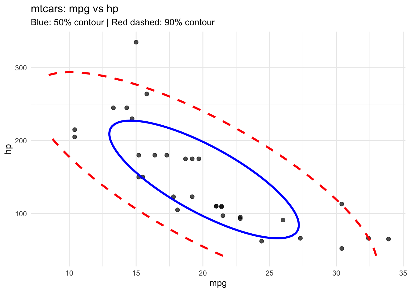

par(mfrow = c(1,2))
qqnorm(X$mpg, main = "Normal Q-Q: mpg"); qqline(X$mpg, col = "blue")
qqnorm(X$hp, main = "Normal Q-Q: hp"); qqline(X$hp, col = "blue")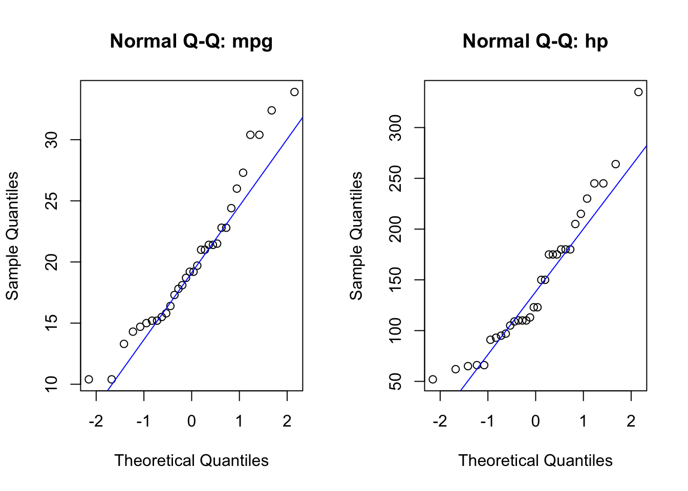

par(mfrow = c(1,1))

sw1 <- shapiro.test(X$mpg)
sw2 <- shapiro.test(X$hp)
cat("Shapiro-Wilk p-value for mpg:", signif(sw1$p.value, 3), "\n")

Shapiro-Wilk p-value for mpg: 0.123 

cat("Shapiro-Wilk p-value for hp:", signif(sw2$p.value, 3), "\n")

Shapiro-Wilk p-value for hp: 0.0488 

# 5. multivariate Shapiro-Wilk test
mvShapiro.Test(as.matrix(X[, c("mpg", "hp")]))

    Generalized Shapiro-Wilk test for Multivariate Normality by
    Villasenor-Alva and Gonzalez-Estrada

data:  as.matrix(X[, c("mpg", "hp")])
MVW = 0.92425, p-value = 0.00639

Interpretation:

• The scatterplot shows the relationship between mpg and hp (likely negative).
• The bivariate normal contours (fit from the data) show the estimated “ellipse” of the joint distribution.
• Q-Q plots help check whether each variable is approximately normal (look for straightness).
• Shapiro-Wilk p-values: p < 0.05 indicates non-normality; p > 0.05 suggests no evidence against normality.
• If either variable is non-normal or the scatterplot is strongly non-elliptical (e.g., curved, outliers), the joint distribution is not truly bivariate normal.

3.7.3 Transformations to Near Normality

If observations show gross departures from normality, it might be necessary to transform some of the variables to near normality. Some recommendations are given below.

Original scale	Transformed scale
Right skewed data	\sqrt{x}   log(x)   1/\sqrt{x}   1/x
x are counts	\sqrt{x}
x are proportions \hat{p}	\mathrm{logit}(\hat{p}) = \frac{1}{2} \log\left(\frac{\hat{p}}{1 - \hat{p}}\right)
x are correlations r	Fisher’s z(r) = \frac{1}{2} \log\left(\frac{1 + r}{1 - r}\right)

3.8 Detecting Outliers

• An outlier is a measurement that appears to be much different from neighboring observations.
• In the univariate case with adequate sample sizes, and assuming that normality holds, an outlier can be detected by:
  • Standardizing the n measurements so that they are approximately N(0, \ 1)
  • Flagging observations with standardized values below or above 3.5 or thereabouts.
• In p dimensions, detecting outliers is not so easy. A sample unit which may not appear to be an outlier in each of the marginal distributions can still be an outlier relative to the multivariate distribution.

3.8.1 Steps for Detecting Outliers

1. Investigate all univariate marginal distributions by computing the standardized values z_{ji} = (x_{ji} - \bar{x}_i) / \sqrt{\sigma_{ii}} for the j-th sample unit and the i-th variable.
2. If p is moderate, construct all bivariate scatter plots. There are p(p-1)/2 of them.
3. For each sample unit, calculate the squared distance d^2_j = (\mathbf{x}_j - \bar{\mathbf{x}})'S^{-1}(\mathbf{x}_j - \bar{\mathbf{x}}), where \mathbf{x}_j is the p \times 1 vector of measurements on the j-th sample unit.
4. To decide if d^2_j is extreme, recall that the d^2_j are approximately \chi^2_p. For example, if n = 100, we would expect to observe about 5 squared distances larger than the 0.95 percentile of the \chi^2_p distribution.

3.8.2 Example: iris Data

library(ggplot2)
library(dplyr)

df = iris
# Bin along x
x_proj <- df %>%
  dplyr::mutate(y = 2)

# Bin along y
y_proj <- df %>%
  mutate(x = 4)

ggplot(df, 
  aes(x = Sepal.Length, 
      y = Sepal.Width, color = Species)) +
  geom_point(size = 1, alpha = 0.7) +
  geom_dotplot(data = x_proj, 
               aes(x = Sepal.Length, y=2, fill = Species),
               binaxis = "x", stackdir = "down", dotsize = 0.5,
               position = position_nudge(y=1.5),
               inherit.aes = FALSE) +
  geom_dotplot(data = y_proj, 
               aes(x=3.5, y = Sepal.Width, fill = Species),
               binaxis = "y", stackdir = "down", dotsize = 0.5,
               position = position_nudge(x=0),
               inherit.aes = FALSE) +
  coord_equal() +
  theme_minimal()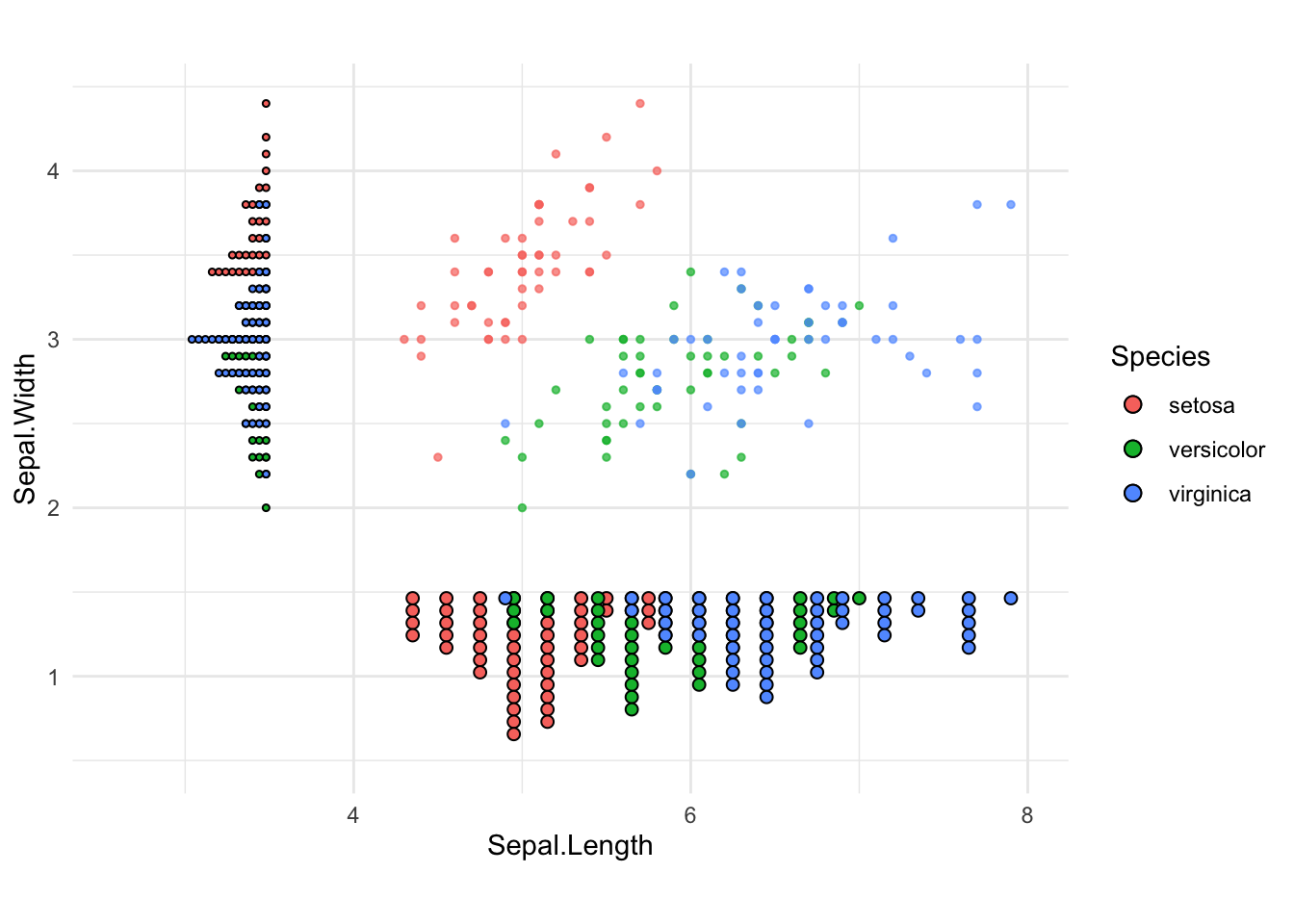

## Finding mahalanobis distance
xbar = colMeans(df[, 1:4])
bvar = cov(df[,1:4])
dsq = mahalanobis(x=df[,1:4], center=xbar, cov=bvar)

## Cutoff value for distances from a chisquare distribution
cutoff = qchisq(p=0.95, df=nrow(bvar)) # 95th percentile 

## plot observations whose distance is greater than cutoff value
flag = dsq>cutoff
cbind(df[flag,1:4], d_sqaure=dsq[flag])

    Sepal.Length Sepal.Width Petal.Length Petal.Width  d_sqaure
16           5.7         4.4          1.5         0.4  9.712790
42           4.5         2.3          1.3         0.3 11.424029
107          4.9         2.5          4.5         1.7 10.137804
115          5.8         2.8          5.1         2.4 11.410573
118          7.7         3.8          6.7         2.2 12.813073
132          7.9         3.8          6.4         2.0 13.101093
135          6.1         2.6          5.6         1.4 12.880331
136          7.7         3.0          6.1         2.3  9.656936
142          6.9         3.1          5.1         2.3 12.441384

# Add flag for outliers
df = df %>%
  mutate(flag = dsq > cutoff)

# Projections
x_proj = df %>% mutate(y = 2)
y_proj = df %>% mutate(x = 4)

ggplot(df, aes(x = Sepal.Length, y = Sepal.Width)) +
  # Scatter plot with flagged points highlighted
  geom_point(aes(color = Species,
                 shape = flag,    # Different shape for flagged
                 size = ifelse(flag, 3, 1.5)), # Larger for flagged
             alpha = 0.7) +
  # X-axis projection
  geom_dotplot(
    data = x_proj,
    aes(x = Sepal.Length, y = 2, fill = Species),
    binaxis = "x", stackdir = "down", binwidth = 0.15, 
    dotsize = 0.5,
    position = position_nudge(y = 1.5),
    inherit.aes = FALSE
  ) +
  # Y-axis projection
  geom_dotplot(
    data = y_proj,
    aes(x = 3.5, y = Sepal.Width, fill = Species),
    binaxis = "y", stackdir = "down", binwidth = 0.15, 
    dotsize = 0.5,
    position = position_nudge(x = 0),
    inherit.aes = FALSE
  ) +
  scale_shape_manual(
    values = c(
      `FALSE` = 16, 
      `TRUE` = 21)) + # open circle for outliers
  scale_size_identity() +
  coord_equal() +
  theme_minimal()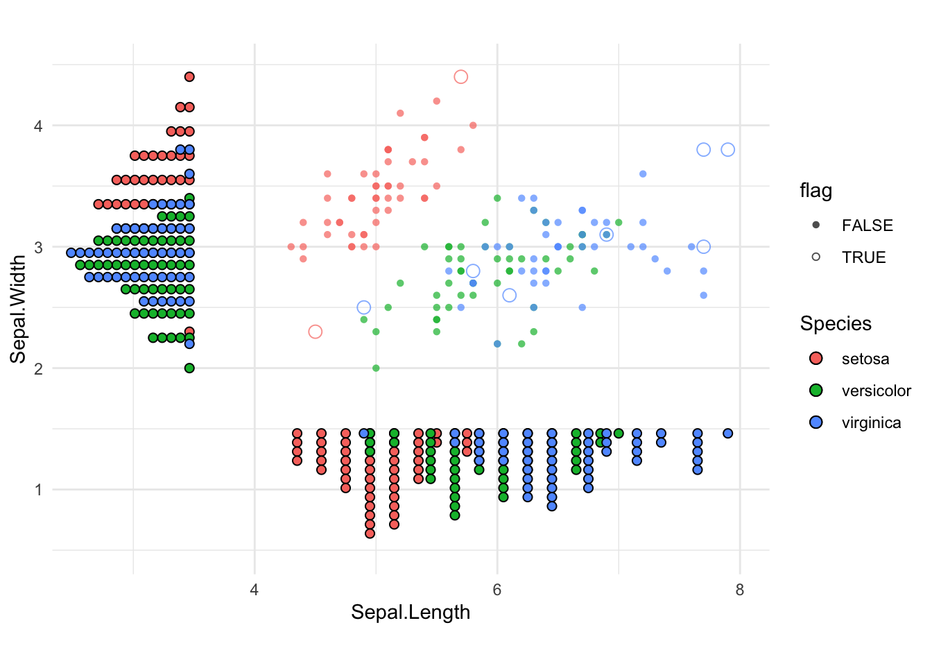

3.9 Exercises

3.9.1 Exercise 1: Perspiration Data

These data were taken from an example in the Johnson and Wichern book, Applied Multivariate Analysis in the file sweat.dat. Three measurements on perspiration were taken from each woman in a random sample of 20 healthy women: X_1= sweat rate, X_2= sodium concentration, X_3=potassium concentration.

• Read the data into R.
• Compute the sample mean and sample covariance
• Treat sample mean and sample covariance as the estimate of population parameters and evaluate the MVN pdf for a range of possible values of variables X_1, X_2.
• Compute the mean and variance of 0.5X_1+ 0.5 X_2 and X_1-X_2.
• Plot the bivariate normal density contour for X_1, X_2 using sample mean and sample covariance.
• Plot a scatterplot with points outside the 95% highlighted.
• Compute Ellipse axes via spectral decomposition.
• Compute generalized variance and total variance based on the whole dataset.
  
• Perform normality check for all the variables.
• Detect any possible outliers at level \alpha =0.05 for all the variables.

View Solution

dat = read.table("sweat.dat", header=F, 
                 col.names=c("subject", "x1", "x2", "x3") )
head(dat)

  subject  x1   x2   x3
1       1 3.7 48.5  9.3
2       2 5.7 65.1  8.0
3       3 3.8 47.2 10.9
4       4 3.2 53.2 12.0
5       5 3.1 55.5  9.7
6       6 4.6 36.1  7.9

X = as.matrix(dat[,c(2,3)])

xbar = colMeans(X)
S = cov(X)
S

          x1       x2
x1  2.879368  10.0100
x2 10.010000 199.7884

grid <- expand.grid(
  x = seq(min(X[,1]) - 0.5, max(X[,1]) + 0.5, length = 50),
  y = seq(min(X[,2]) - 0.5, max(X[,2]) + 0.5, length = 50)
)
gridmat = as.matrix(grid)
dens <- mvtnorm::dmvnorm(x=gridmat, 
                         mean = xbar, 
                         sigma = S)
head(data.frame(grid, f = dens))

         x  y            f
1 1.000000 13 0.0002244281
2 1.163265 13 0.0002563175
3 1.326531 13 0.0002894749
4 1.489796 13 0.0003232772
5 1.653061 13 0.0003570021
6 1.816327 13 0.0003898505

# mean, var
a1 = c(0.5, 0.5)
a2 = c(1, -1)

# mean and variance of 0.5*X1 + 0.5*X2
tibble(
  mean = sum(a1 * xbar),
  variance = drop(t(a1) %*% S %*% a1)
)

# A tibble: 1 × 2
   mean variance
  <dbl>    <dbl>
1  25.0     55.7

# mean and variance of X1 - X2
tibble(
  mean = sum(a2 * xbar),
  variance = drop(t(a2) %*% S %*% a2)
)

# A tibble: 1 × 2
   mean variance
  <dbl>    <dbl>
1 -40.8     183.

grid$z = dens 
ggplot(grid, aes(x = x, y = y, z = z)) +
  geom_contour_filled(bins = 10) +
  #coord_equal() +
  labs(title = "Bivariate Normal Density (Contours)",
       x = "Sweat rate", y = "Sodium concentration", 
       fill = "Density") +
  theme_minimal()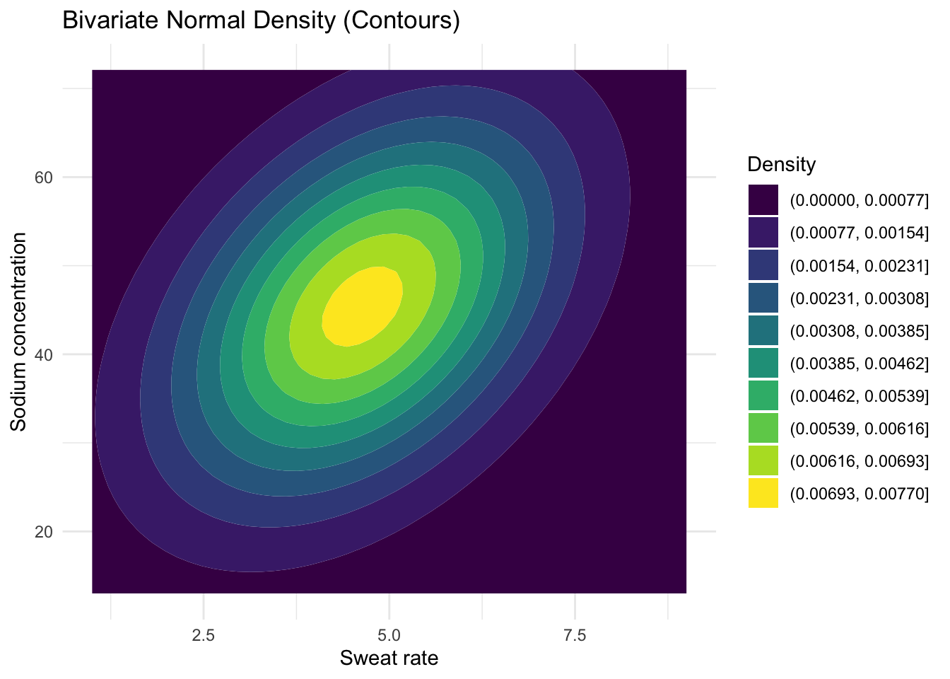

Xc = X - matrix(1, nrow=nrow(X), ncol=1) %*% t(xbar)
Q = diag( Xc %*% solve(S) %*% t(Xc) )
# or use T2 = rowSums( (Xc %*% solve(S)) * Xc)
cut = qchisq(.95, df=2)
mean(Q<=cut) # empirical coverage 

[1] 0.95

dat1 = as.data.frame(X) %>% 
  mutate(inside = Q<=cut)
ggplot(dat1, aes(x=x1, y=x2, color=inside)) + 
  geom_point(size=2, alpha=.8) + 
  scale_color_manual(values = c("FALSE"="grey60",
                                "TRUE"="tomato")) + 
  labs(color = "Inside 95% ellipse?")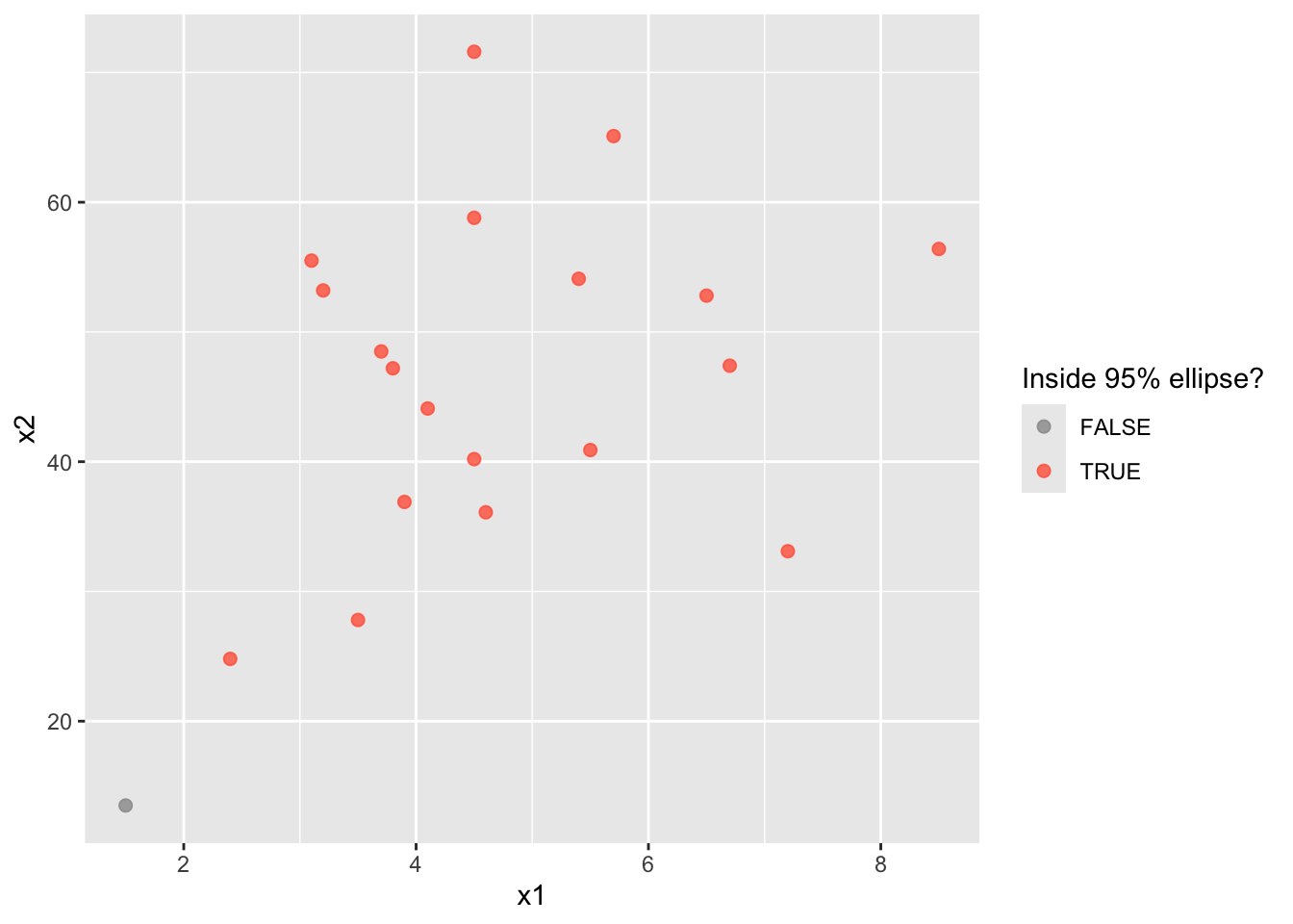

E = eigen(S)

# Ellipse directions
E$vectors

          [,1]       [,2]
[1,] 0.0506399 -0.9987170
[2,] 0.9987170  0.0506399

# lengths
sqrt(E$values) * sqrt(cut)

[1] 34.641972  3.769698

tibble(
  "Generalized variance" = prod(E$values),
  "Total variance" = sum(E$values)
)

# A tibble: 1 × 2
  `Generalized variance` `Total variance`
                   <dbl>            <dbl>
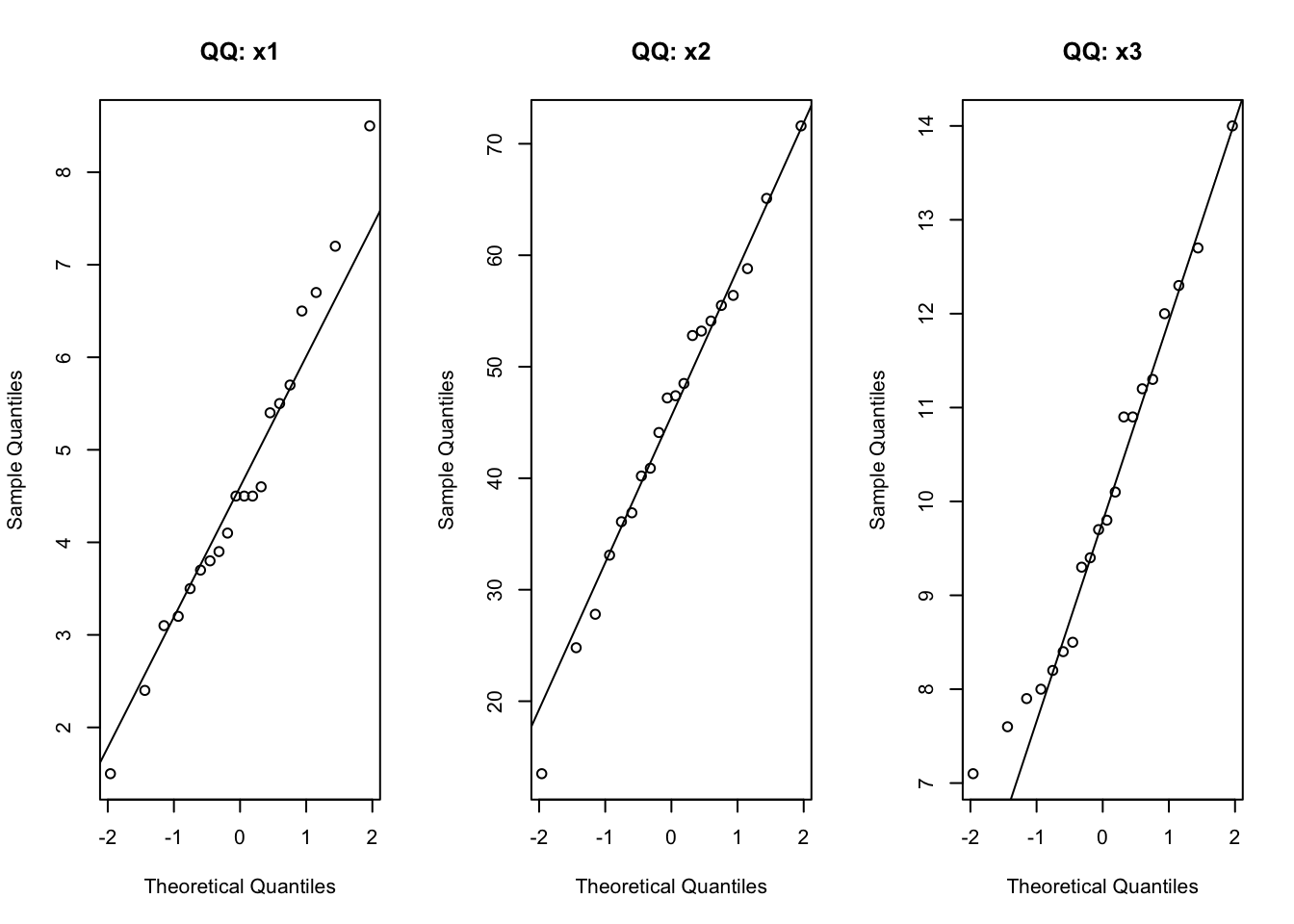
1                   475.             203.

par(mfrow = c(1,3))
for (nm in colnames(dat[,2:4])) {
  qqnorm(dat[, nm], main = paste("QQ:", nm))
  qqline(dat[, nm])
}

par(mfrow = c(1,1))

apply(dat[, 2:4], 2, function(v) shapiro.test(v)$p.value)

       x1        x2        x3 
0.8689242 0.9861883 0.6232620 

mvShapiroTest::mvShapiro.Test(as.matrix(dat[,2:4]))

    Generalized Shapiro-Wilk test for Multivariate Normality by
    Villasenor-Alva and Gonzalez-Estrada

data:  as.matrix(dat[, 2:4])
MVW = 0.94446, p-value = 0.2567

dat1 = as.matrix(dat[,2:4])
xbar1 = colMeans(dat1)
S1 = cov(dat1)
Xc1 = dat1 - matrix(1,nrow(dat1), 1) %*% t(xbar1)
d2 = diag( (Xc1) %*% solve(S1) %*% t(Xc1) )

cut2 = qchisq(.975, df=ncol(dat1))
sum(d2>cut2)

[1] 0