1 Introduction to Multivariate Data

Author

Pulong Ma

1.1 Course Outline

Introduction to Multivariate Data
Numerical Summaries and Visualization of Multivariate Data
Multivariate Normal Distribution
Comparing Centers of Distributions
(Hotelling T^2, MANOVA, Repeated Measures)
Principal Component Analysis
(Summarizing data in lower dimensions)
Exploratory Factor Analysis
(What to do when the variables of interest cannot be directly observed.)
Multi-Dimensional Scaling
Cluster Analysis
Discriminant Analysis and Classification
(Including linear discriminants, logistic regression, classification trees, and random forests)

1.2 Objectives of Multivariate Analysis

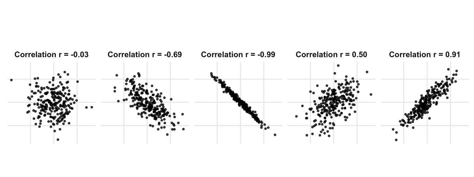
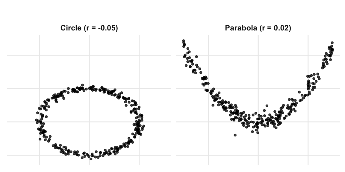
Understand dependencies among variables: What is the nature of associations among variables?
Prediction: If variables are associated, then we might be able to predict the value of some of them given information on the others. (Statistical inference)
Hypothesis testing: Are differences in sets of response means for two or more groups large enough to be distinguished from sampling variation? (Statistical inference)
Dimensionality reduction: Can we reduce the dimensionality of the problem by considering a small number of (linear) combinations of a large number of measurements without losing important information?
- Principal Components
- Factor Analysis
- Multidimensional Scaling
Grouping (Cluster Analysis): Identify groups of “similar” units using a common set of measured traits.
Classification: Classify units into previously defined groups using a common set of measured traits.

1.3 Introduction to R and RStudio

1.3.1 Getting Started

To download R, please choose your preferred CRAN mirror. Here I recommend the mirror 0-Cloud available at https://cloud.r-project.org/.

Install R on macOS

For macOS users, below are the steps you need to install R.

Install Xcode (e.g., via the App Store). Skip this step if your Mac already has Xcode installed.
Install XQuartz.
Go to https://cloud.r-project.org/ and click “Download R for macOS.”
Click on the download link for the latest R version for macOS and follow the instruction.

Install R on Windows:

For Windows users, the following instructions guide you to install R.

Go to https://cloud.r-project.org/ and click “Download R for Windows.”
Click “install R for the first time.”
Choose a download mirror (any CRAN mirror will work).
Click on the download link for the latest R version for Windows and follow the instruction

Install RStudio

RStudio has multiple panes in the window, open by default: one for writing and editing code, another for executing it, another for plots produced or help, and another that lists the R data objects available. RStudio can be download for free at https://posit.co/download/rstudio-desktop/.

1.3.2 Introduction to R Programming

Some Tips: R Working Environment

Whenever you work with R for data analysis, it is recommended to load all the packages used in the data analysis pipeline before the function sessionInfo(). In addition, if random numbers are generated, it is also recommended to set random seed to ensure reproducibility using set.seed().

R Working Environment

# load packages 
library(ggplot2)
library(tidyr)
library(dplyr)
library(readr)
library(lubridate)

sessionInfo()

R version 4.4.3 (2025-02-28)
Platform: aarch64-apple-darwin20
Running under: macOS Sequoia 15.3.2

Matrix products: default
BLAS:   /Library/Frameworks/R.framework/Versions/4.4-arm64/Resources/lib/libRblas.0.dylib 
LAPACK: /Library/Frameworks/R.framework/Versions/4.4-arm64/Resources/lib/libRlapack.dylib;  LAPACK version 3.12.0

locale:
[1] en_US.UTF-8/en_US.UTF-8/en_US.UTF-8/C/en_US.UTF-8/en_US.UTF-8

time zone: America/Chicago
tzcode source: internal

attached base packages:
[1] stats     graphics  grDevices utils     datasets  methods   base     

other attached packages:
[1] lubridate_1.9.4 readr_2.1.5     tidyr_1.3.1     dplyr_1.1.4    
[5] ggplot2_3.5.2  

loaded via a namespace (and not attached):
 [1] vctrs_0.6.5        cli_3.6.5          knitr_1.50         rlang_1.1.6       
 [5] xfun_0.52          purrr_1.0.4        generics_0.1.4     jsonlite_2.0.0    
 [9] glue_1.8.0         htmltools_0.5.8.1  hms_1.1.3          scales_1.4.0      
[13] rmarkdown_2.29     grid_4.4.3         evaluate_1.0.3     tibble_3.2.1      
[17] tzdb_0.5.0         fastmap_1.2.0      yaml_2.3.10        lifecycle_1.0.4   
[21] compiler_4.4.3     RColorBrewer_1.1-3 timechange_0.3.0   htmlwidgets_1.6.4 
[25] pkgconfig_2.0.3    rstudioapi_0.17.1  farver_2.1.2       digest_0.6.37     
[29] R6_2.6.1           tidyselect_1.2.1   pillar_1.10.2      magrittr_2.0.3    
[33] withr_3.0.2        tools_4.4.3        gtable_0.3.6

R is a Calculator

Code

# Numeric, logical, character types
3.14159             # numeric

[1] 3.14159

Code

T                   # logical, can also be TRUE

[1] TRUE

Code

F                   # logical, can also be FALSE

[1] FALSE

Code

"Stat 4750/5750"    # character

[1] “Stat 4750/5750”

Code

# Basic arithmetic operators
1 + 2

[1] 3

Code

20 - 3

[1] 17

Code

2 * 6

[1] 12

Code

4 / 3

[1] 1.333333

Code

2 ^ 4

[1] 16

Code

-3.14

[1] -3.14

Code

(1 + 2) * (3 / 4)  # use parenthesis

[1] 2.25

Code

2 == 1

[1] FALSE

Code

# Vector
c()  # empty vector

NULL

Code

c(1, 2, 3, 4)

[1] 1 2 3 4

Code

1:4

[1] 1 2 3 4

Code

# Look up the function help, 3 ways:
# Following 3 ways work for most functions
          # 1. search in help pane
?sum      # 2. use ?
sum(1:4)  # 3. move your cursor to the function, then press F1, the easiest way

[1] 10

Code

# The 3rd way doesn't work for functions having some symbols, like +, ==, %*%
          # 1. search in help pane
?`+`      # 2. use ? but wrap the symbol with ``

R Objects

Code

# Assignment operator <-

# Numeric class
mynumbers <- 5:12
mynumbers

[1]  5  6  7  8  9 10 11 12

Code

mynumbers + 2

[1]  7  8  9 10 11 12 13 14

Code

mynumbers * 10

[1]  50  60  70  80  90 100 110 120

Code

typeof(mynumbers)      # type of an object

[1] "integer"

Code

# check if is numeric (both integer and double type are numeric)
is.numeric(mynumbers)

[1] TRUE

Code

is.vector(mynumbers)   # check if is vector

[1] TRUE

Code

length(mynumbers)      # length of an object

[1] 8

Code

# Character class
mytext <- c("hello", "class", "four") 
mytext

[1] "hello" "class" "four"

Code

typeof(mytext)

[1] "character"

Code

is.numeric(mytext)

[1] FALSE

Code

is.character(mytext)

[1] TRUE

Code

is.character(mynumbers)

[1] FALSE

Code

is.vector(mytext)

[1] TRUE

Code

length(mytext)

[1] 3

Code

# Logical class
mylogic <- c(TRUE, FALSE, TRUE, TRUE)
typeof(mylogic)

[1] "logical"

Code

# Factor class
gender <- c("male", "female", "female", "female", "male") 
gender

[1] "male"   "female" "female" "female" "male"

Code

is.vector(gender)

[1] TRUE

Code

is.character(gender)

[1] TRUE

Code

is.vector(gender)

[1] TRUE

Code

is.factor(gender)

[1] FALSE

Code

genderf <- factor(gender)
genderf

[1] male   female female female male  
Levels: female male

Code

is.character(genderf)

[1] FALSE

Code

is.factor(genderf)

[1] TRUE

Code

summary(mynumbers)  # numeric: 5-number summary

   Min. 1st Qu.  Median    Mean 3rd Qu.    Max. 
   5.00    6.75    8.50    8.50   10.25   12.00

Code

summary(mylogic)    # logical: count how many T and F

   Mode   FALSE    TRUE 
logical       1       3

Code

summary(mytext)     # character:

   Length     Class      Mode 
        3 character character

Code

summary(genderf)    # factor: count the frequency

female   male 
     3      2

Code

# List class
mylist <- list(1, "ABC", FALSE)
mylist

[[1]]
[1] 1

[[2]]
[1] "ABC"

[[3]]
[1] FALSE

Code

is.vector(mylist)

[1] TRUE

Code

is.list(mylist)

[1] TRUE

Code

length(mylist)

[1] 3

Working with Matrices

Code

# All elements should be the same type
mydata <- matrix(c(140, 120, 160, 145, 125, 65, 60, 63, 66, 61), ncol = 2, byrow = FALSE) 
mydata

     [,1] [,2]
[1,]  140   65
[2,]  120   60
[3,]  160   63
[4,]  145   66
[5,]  125   61

Code

dim(mydata)  # dimensions

[1] 5 2

Code

colnames(mydata) <- c("Weight.lbs", "Height.in")
rownames(mydata) <- c("a", "b", "c", "d", "e")
mydata

  Weight.lbs Height.in
a        140        65
b        120        60
c        160        63
d        145        66
e        125        61

Code

summary(mydata)  # summary of each column

   Weight.lbs    Height.in 
 Min.   :120   Min.   :60  
 1st Qu.:125   1st Qu.:61  
 Median :140   Median :63  
 Mean   :138   Mean   :63  
 3rd Qu.:145   3rd Qu.:65  
 Max.   :160   Max.   :66

Working with Data Frames

Data Frames

# Different columns can have different types
df <- data.frame(Weight.lbs = c(140, 120, 160, 145, 125, 180, 165),
                 Height.in = c(65, 60, 63, 66, 61, 70, 68),
                 Gender = c(rep("Female", 5), rep("Male", 2)), stringsAsFactors = T)
df

  Weight.lbs Height.in Gender
1        140        65 Female
2        120        60 Female
3        160        63 Female
4        145        66 Female
5        125        61 Female
6        180        70   Male
7        165        68   Male

Data Frames

dim(df)

[1] 7 3

Data Frames

head(df)     # the first 6 rows

  Weight.lbs Height.in Gender
1        140        65 Female
2        120        60 Female
3        160        63 Female
4        145        66 Female
5        125        61 Female
6        180        70   Male

Data Frames

summary(df)  # summary of each column

   Weight.lbs      Height.in        Gender 
 Min.   :120.0   Min.   :60.00   Female:5  
 1st Qu.:132.5   1st Qu.:62.00   Male  :2  
 Median :145.0   Median :65.00             
 Mean   :147.9   Mean   :64.71             
 3rd Qu.:162.5   3rd Qu.:67.00             
 Max.   :180.0   Max.   :70.00

Data Frames

str(df)      # structure of the data frame

'data.frame':   7 obs. of  3 variables:
 $ Weight.lbs: num  140 120 160 145 125 180 165
 $ Height.in : num  65 60 63 66 61 70 68
 $ Gender    : Factor w/ 2 levels "Female","Male": 1 1 1 1 1 2 2

a tibble is a modern implementation of a data frame, designed to be more user-friendly and efficient, especially when working with large datasets.

tibble

# install.packages("tibble")
library(tibble)
# create a tibble from an existing object
as_tibble(df)

# A tibble: 7 × 3
  Weight.lbs Height.in Gender
       <dbl>     <dbl> <fct> 
1        140        65 Female
2        120        60 Female
3        160        63 Female
4        145        66 Female
5        125        61 Female
6        180        70 Male  
7        165        68 Male

tibble

# create a new tibble 
tibble(x=1:5, 
       y=1.0,
       z=x^2+y)

# A tibble: 5 × 3
      x     y     z
  <int> <dbl> <dbl>
1     1     1     2
2     2     1     5
3     3     1    10
4     4     1    17
5     5     1    26

tibble

# define a row-by-row tibble
tribble(
  ~x, ~y, ~z,
  "a", 2, 1,
  "b", 3, 4
)

# A tibble: 2 × 3
  x         y     z
  <chr> <dbl> <dbl>
1 a         2     1
2 b         3     4

Operations on Matrix and Data Frame

Code

mydata[, 1]                     # extract the first column

  a   b   c   d   e 
140 120 160 145 125

Code

mydata[1, ]                     # extract the first row

Weight.lbs  Height.in 
       140         65

Code

mydata[1:2, ]                   # extract the first two rows

  Weight.lbs Height.in
a        140        65
b        120        60

Code

mydata[3, 2]                    # extract the element in the third row and the second column

[1] 63

Code

df[seq(1, 7, 2), ]              # extract every second row

  Weight.lbs Height.in Gender
1        140        65 Female
3        160        63 Female
5        125        61 Female
7        165        68   Male

Code

seq(1, 7, 2)

[1] 1 3 5 7

Code

subset(df, Gender == "Male")    # select based on value

  Weight.lbs Height.in Gender
6        180        70   Male
7        165        68   Male

Code

t(mydata)                       # transpose of matrix

             a   b   c   d   e
Weight.lbs 140 120 160 145 125
Height.in   65  60  63  66  61

Code

mydata[, 1] * mydata[, 2]       # element-wise multiplication

    a     b     c     d     e 
 9100  7200 10080  9570  7625

Code

mydata %*% t(mydata)            # matrix multiplication

      a     b     c     d     e
a 23825 20700 26495 24590 21465
b 20700 18000 22980 21360 18660
c 26495 22980 29569 27358 23843
d 24590 21360 27358 25381 22151
e 21465 18660 23843 22151 19346

Plotting with the ggplot2 Package

Code

library(ggplot2)
data("USArrests")
dat = USArrests %>% as_tibble()
dat %>% 
  ggplot(aes(x=UrbanPop, y=Murder)) + 
  geom_point()

Code

dat_long = dat %>%
  tidyr::pivot_longer(1:4,names_to = "Variable", values_to = "Value") 
head(dat_long)

# A tibble: 6 × 2
  Variable Value
  <chr>    <dbl>
1 Murder    13.2
2 Assault  236  
3 UrbanPop  58  
4 Rape      21.2
5 Murder    10  
6 Assault  263

Code

# faceted histogram
ggplot(dat_long, aes(Value)) + 
  geom_histogram(bins=20, fill="grey80", color="white") + 
  facet_wrap(~Variable, scales="free") + 
  labs(title = "Distributions by Variable")

1.4 Organization of Data and Notation

n = the number of observations or units
p = the number of variables measured on each unit
If p = 1, then we are back in the usual univariate setting
x_{ik} = the i-th observation of the k-th variable

\text{Observations} \quad \overset{\text{Variables}}{ \begin{bmatrix} x_{11} & x_{12} & \cdots & x_{1p} \\ x_{21} & x_{22} & \cdots & x_{2p} \\ \vdots & \vdots & \ddots & \vdots \\ x_{n1} & x_{n2} & \cdots & x_{np} \end{bmatrix} }

Data matrix: X_{n \times p}=\left[ \begin{array}{cccc} x_{11} & x_{12} & \cdots & x_{1p} \\ x_{21} & x_{22} & \cdots & x_{2p} \\ \vdots & \vdots & & \vdots \\ x_{n1} & x_{n2} & \cdots & x_{np}\end{array} \right ]
This can be written as n rows or as p columns X_{n \times p} = \begin{bmatrix} \mathbf{x}_1^{\prime} \\ \mathbf{x}_2^{\prime} \\ \vdots \\ \mathbf{x}_n^{\prime} \end{bmatrix} = \begin{bmatrix} \mathbf{x}_1^{\top} \\ \mathbf{x}_2^{\top} \\ \vdots \\ \mathbf{x}_n^{\top} \end{bmatrix} = \left[ \mathbf{x}_1, \mathbf{x}_2, \ldots, \mathbf{x}_p \right] where both \prime and \top represent matrix transpose.

R Code: Data Organization

X = as.matrix(USArrests)
dim(X)

[1] 50  4

R Code: Matrix Transpose

t(X[1:5,])

         Alabama Alaska Arizona Arkansas California
Murder      13.2   10.0     8.1      8.8        9.0
Assault    236.0  263.0   294.0    190.0      276.0
UrbanPop    58.0   48.0    80.0     50.0       91.0
Rape        21.2   44.5    31.0     19.5       40.6

1.5 Descriptive Statistics

1.5.1 Sample Mean

The sample mean of the kth variable (k = 1,...,p) is \bar{x}_k = \frac{1}{n} \sum_{i = 1}^n x_{ik}

1.5.2 Sample Variance and Sample Standard Deviation

The sample variance of the kth variable is s^2_k = \frac{1}{n-1} \sum_{i=1}^n (x_{ik} - \bar{x}_k)^2
The sample standard deviation is given by s_k = \sqrt{s^2_k}
We often use s_{kk} to denote the sample variance for the k-th variable. Thus, s^2_k = s_{kk}

1.5.3 Sample Covariance and Sample Correlation

The sample covariance between variable k and variable j is computed as s_{jk} = \frac{1}{n-1} \sum_{i=1}^n (x_{ij} - \bar{x}_j) (x_{ik} - \bar{x}_k)
If variables k and j are independent, the population covariance will be exactly zero, but the sample covariance will vary about zero.
The sample correlation between variables k and j is defined as r_{jk} = \frac{s_{jk}}{\sqrt{s_{jj}} \sqrt{s_{kk}}}
r_{jk} is between -1 and 1.
r_{jk} = r_{kj}
The sample correlation is equal to the sample covariance if measurements are standardized.
The sample correlation (r_{ij}) will vary about the value of the population correlation (\rho_{ij})

R Code: Descriptive Statistics

# load built-in US crime rates data
data("USArrests") 
dat = USArrests 
head(dat)

           Murder Assault UrbanPop Rape
Alabama      13.2     236       58 21.2
Alaska       10.0     263       48 44.5
Arizona       8.1     294       80 31.0
Arkansas      8.8     190       50 19.5
California    9.0     276       91 40.6
Colorado      7.9     204       78 38.7

Sample mean

mu = colMeans(dat)
mu

  Murder  Assault UrbanPop     Rape 
   7.788  170.760   65.540   21.232

Sample mean

library(dplyr)
dat %>% 
  summarise(across(where(is.numeric), mean))

  Murder Assault UrbanPop   Rape
1  7.788  170.76    65.54 21.232

Sample variance

s2 = apply(dat, 2, var)
s2

    Murder    Assault   UrbanPop       Rape 
  18.97047 6945.16571  209.51878   87.72916

Sample variance

# using dplyr
dat %>% 
  summarise(across(where(is.numeric), var))

    Murder  Assault UrbanPop     Rape
1 18.97047 6945.166 209.5188 87.72916

Sample standard deviation

# compute standard deviation from data 
s = apply(dat, 2, sd)  
# or from sample variance 
s = sqrt(s2)
s

   Murder   Assault  UrbanPop      Rape 
 4.355510 83.337661 14.474763  9.366385

Sample covariance

n = nrow(dat)
s_jk = 1/(n-1) * sum((dat[,1] - mu[1]) * (dat[,2] - mu[2]))
s_jk

[1] 291.0624

Sample correlation

r_jk = s_jk / sqrt(s2[1] * s2[2])

1.5.4 Covariance and Correlation Measures

Covariance and correlation measure linear association.
Other non-linear (or curved) relationships may exist among variables even if r_{jk} = 0.
A population correlation of zero means no linear association,
but it does not necessarily imply independence.

Nonlinear Dependence with (Near) Zero Correlation

1.6 Matrix Organization of Descriptive Statistics

1.6.1 Sample Mean

Sample mean: \bar{\mathbf{x}} is the p \times 1 vector of sample means:

\bar{\mathbf{x}} = \begin{bmatrix} \bar{x}_1 \\ \bar{x}_2 \\ \vdots \\ \bar{x}_p \end{bmatrix}

\bar{\mathbf{x}} is an estimate of the vector of population means:

\boldsymbol{\mu} = \begin{bmatrix} \mu_1 \\ \mu_2 \\ \vdots \\ \mu_p \end{bmatrix}

R Code: Sample Mean

X = as.matrix(USArrests)
xbar = colMeans(X)
xbar

  Murder  Assault UrbanPop     Rape 
   7.788  170.760   65.540   21.232

Centered Data: X_c = X - \mathbf{1}_n \bar{\mathbf{x}}^\top

R Code: Centered Data

n = nrow(X) 
ones_n = matrix(1, n, ncol=1)
Xc = X - ones_n %*% t(xbar)

1.6.2 Sample Covariance

S is the p \times p symmetric matrix of sample variances (on the diagonal) and sample covariances (the off-diagonal elements):

S = \begin{bmatrix} s_{11} & s_{12} & s_{13} & \cdots & s_{1p} \\ s_{21} & s_{22} & s_{23} & \cdots & s_{2p} \\ \vdots & \vdots & \vdots & & \vdots \\ s_{p1} & s_{p2} & s_{p3} & \cdots & s_{pp} \end{bmatrix} = \frac{1}{n-1} \sum_{i=1}^n (\mathbf{x}_i - \bar{\mathbf{x}})(\mathbf{x}_i - \bar{\mathbf{x}})^{\top} = \frac{1}{n-1} X_c^\top X_c

S is an estimate of the population covariance matrix:

\Sigma = \begin{bmatrix} \sigma_{11} & \sigma_{12} & \sigma_{13} & \cdots & \sigma_{1p} \\ \sigma_{21} & \sigma_{22} & \sigma_{23} & \cdots & \sigma_{2p} \\ \vdots & \vdots & \vdots & & \vdots \\ \sigma_{p1} & \sigma_{p2} & \sigma_{p3} & \cdots & \sigma_{pp} \end{bmatrix}

R Code: Sample Covariance

S = cov(X) 
# or using matrix algebra
S_mat = t(Xc)%*%Xc/(n-1)
signif(cbind(S, S_mat),4)

          Murder Assault UrbanPop   Rape  Murder Assault UrbanPop   Rape
Murder    18.970   291.1    4.386  22.99  18.970   291.1    4.386  22.99
Assault  291.100  6945.0  312.300 519.30 291.100  6945.0  312.300 519.30
UrbanPop   4.386   312.3  209.500  55.77   4.386   312.3  209.500  55.77
Rape      22.990   519.3   55.770  87.73  22.990   519.3   55.770  87.73

1.6.3 Sample Correlation

The p \times p matrix of sample correlations is also symmetric:

R = \begin{bmatrix} 1 & r_{12} & r_{13} & \cdots & r_{1p} \\ r_{21} & 1 & r_{23} & \cdots & r_{2p} \\ \vdots & \vdots & \vdots & & \vdots \\ r_{p1} & r_{p2} & r_{p3} & \cdots & 1 \end{bmatrix} = D^{-1/2} \, S \, D^{-1/2}

D^{-1/2} is a diagonal matrix with (j,j) entry 1/\sqrt{s_{jj}} = 1/s_j, i.e.,

D^{-1/2} = \begin{bmatrix} \frac{1}{\sqrt{s_{11}}} & 0 & 0 & \cdots & 0 \\ 0 & \frac{1}{\sqrt{s_{22}}} & 0 & \cdots & 0 \\ \vdots & \vdots & \vdots & & \vdots \\ 0 & 0 & 0 & \cdots & \frac{1}{\sqrt{s_{pp}}} \end{bmatrix}

R is an estimate of the population correlation matrix P = \begin{bmatrix} 1 & \rho_{12} & \rho_{13} & \cdots & \rho_{1p} \\ \rho_{21} & 1 & \rho_{23} & \cdots & \rho_{2p} \\ \vdots & \vdots & \vdots & & \vdots \\ \rho_{p1} & \rho_{p2} & \rho_{p3} & \cdots & 1 \end{bmatrix}

R Code: Sample Correlation

R = cor(X)
R

             Murder   Assault   UrbanPop      Rape
Murder   1.00000000 0.8018733 0.06957262 0.5635788
Assault  0.80187331 1.0000000 0.25887170 0.6652412
UrbanPop 0.06957262 0.2588717 1.00000000 0.4113412
Rape     0.56357883 0.6652412 0.41134124 1.0000000

R Code: Pairwise Scatterplots and Correlations

GGally::ggpairs(dat)

1.7 Standardization

1.7.1 Standardized Data (or z-Scores)

Suppose x_{ij} is the measurement on the j-th outcome variable for the i-th subject in the data set.
The standardized value is
z_{ij} = \frac{x_{ij} - \bar{x}_{j}}{s_j}
The entire set of p standardized responses for the i-th subject can be computed as
\mathbf{z}_i = \begin{bmatrix} z_{i1} \\ z_{i2} \\ \vdots \\ z_{ip} \end{bmatrix} = \begin{bmatrix} \dfrac{x_{i1} - \bar{x}_{1}}{s_1} \\ \dfrac{x_{i2} - \bar{x}_{2}}{s_2} \\ \vdots \\ \dfrac{x_{ip} - \bar{x}_{p}}{s_p} \end{bmatrix} = D^{-1/2} (\mathbf{x}_i - \bar{\mathbf{x}})

R Code: Standardized Data

s_j = sqrt(diag(S))

Dsqrt = diag(1/s_j)

# using matrix algebra
Z =  (X -  matrix(1, nrow(X), 1) %*% matrix(xbar, 1)) %*% Dsqrt

# using scale function 
X_scaled = as.matrix(scale(X, center=TRUE, scale=TRUE))


# using mutate function
dat_scaled <- dat %>%
  mutate(across(everything(), ~ (.x - mean(.x)) / sd(.x)))

R Code: Plotting the Data

p1 = ggplot(dat, aes(Murder, Assault)) + 
  geom_point(alpha=0.8) + 
  labs(title="Unscaled")

p2 = ggplot(dat_scaled, aes(Murder, Assault)) + 
  geom_point(alpha=.8) + 
  labs(title="Standardized (z-scores)")

patchwork::wrap_plots(p1, p2, ncol=1)

1.7.2 Standardized Population Mean

The vector of true means for a set of standardized responses is
a vector of zeros:

E(\mathbf{z}_i) = E\begin{bmatrix} z_{i1} \\ z_{i2} \\ \vdots \\ z_{ip} \end{bmatrix} = E\begin{bmatrix} \dfrac{x_{i1} - \bar{x}_{1}}{s_1} \\ \dfrac{x_{i2} - \bar{x}_{2}}{s_2} \\ \vdots \\ \dfrac{x_{ip} - \bar{x}_{p}}{s_p} \end{bmatrix} = \begin{bmatrix} 0 \\ 0 \\ \vdots \\ 0 \end{bmatrix}

The vector of estimated means for a set of standardized responses
is also a vector of zeros.

1.7.3 Standardized Population Covariance

The true covariance matrix for a set of standardized responses is the population correlation matrix:

\text{Var}(\mathbf{z}_i) = P = \begin{bmatrix} 1 & \rho_{12} & \cdots & \rho_{1p} \\ \rho_{21} & 1 & \cdots & \rho_{2p} \\ \vdots & \vdots & \ddots & \vdots \\ \rho_{p1} & \rho_{p2} & \cdots & 1 \end{bmatrix}

An estimate of the true covariance matrix for a set of standardized responses is the sample correlation matrix:

\widehat{\text{Var}(\mathbf{z}_i)} = R = \begin{bmatrix} 1 & r_{12} & \cdots & r_{1p} \\ r_{21} & 1 & \cdots & r_{2p} \\ \vdots & \vdots & \ddots & \vdots \\ r_{p1} & r_{p2} & \cdots & 1 \end{bmatrix} = D^{-1/2} S D^{-1/2}

1.8 Exercises

1.8.1 Exercise 1: Data Types

Common types of objects for data analysis are numeric, character, logical, factors, and dates. Character data do not have numerical values, such as names of people or words in a book, Logical data takes values of true or false and can be used to make decisions.

For each of the following commands, either explain why they should be errors, or explain the non-erroneous result.

    x <- c("1","2","3")
    max(x)
    sort(x)
    sum(x)

For the next two commands, either explain their results, or why they should produce errors.

    y <- c("1",3,4)
    y[2] + y[3]

For the next two commands, either explain their results, or why they should produce errors.

    z <- data.frame(z1="1", z2=3, z3=5)
    z[1,2] + z[1,3]

View Solution

x is bound to a vector of characters instead of numerical values. The functions max, sort, sum should take numerical values as input, so the values in x are first converted from characters to numerical values implicitly and then the functions apply to these incorrect numerical values
y is a vector of characters, which cannot be used for addition
z is a data frame, but the variable z1 is a character while z2 and z3 are numerical. Adding z2 and z3 will produce the correct results.

1.8.2 Exercise 2: Working with Matrix and Data Frames

A matrix is a 2D array, with rows and columns, much like you would have seen in linear algebra. Primarily we think of these as numeric objects. Arrays can have more than two dimensions. In multivariate analysis we are typically thinking of data in the form of a matrix, with samples/cases in the rows and variables represented as columns. Data frames are 2D arrays that could have multiple types of data in different columns. Lists are collections of possibly different length and different types of objects.

Create a matrix and print it out.

View Solution

dat = matrix(c(140, 120, 160, 145, 125, 
               65, 60, 63, 66, 61), 
             ncol = 2, byrow = FALSE)

View Solution

dat # or print(dat)

     [,1] [,2]
[1,]  140   65
[2,]  120   60
[3,]  160   63
[4,]  145   66
[5,]  125   61

Rename the column names of a matrix.

View Solution

colnames(dat) = c("weight.lbs", "Height.in")
dat

     weight.lbs Height.in
[1,]        140        65
[2,]        120        60
[3,]        160        63
[4,]        145        66
[5,]        125        61

Data frames can store both columns of numeric data and columns of character data, columns of integers, and factors.

Create a data frame with Male and Female observations, and print out the data frame.

View Solution

df = data.frame(
  Weight.lbs = c(140, 120, 160, 145, 125,
       180, 165), 
  Height.in = c(65, 60, 63, 66, 61, 70, 68),
  Gender = c(rep("Female", 5), rep("Male", 2))
  ) 

df

  Weight.lbs Height.in Gender
1        140        65 Female
2        120        60 Female
3        160        63 Female
4        145        66 Female
5        125        61 Female
6        180        70   Male
7        165        68   Male

Get the rows and columns of a data frame.

View Solution

dim(df)

[1] 7 3

View Solution

nrow(df)

[1] 7

View Solution

ncol(df)

[1] 3

Get summary statistics of a data frame.

View Solution

summary(df)

   Weight.lbs      Height.in        Gender         
 Min.   :120.0   Min.   :60.00   Length:7          
 1st Qu.:132.5   1st Qu.:62.00   Class :character  
 Median :145.0   Median :65.00   Mode  :character  
 Mean   :147.9   Mean   :64.71                     
 3rd Qu.:162.5   3rd Qu.:67.00                     
 Max.   :180.0   Max.   :70.00

Operations with Matrix and Data Frame

Extract the first row and second column of a matrix.

View Solution

dat[1,]

weight.lbs  Height.in 
       140         65

View Solution

dat[,2]

[1] 65 60 63 66 61

Subset the first two rows of a matrix

View Solution

dat[1:2,]

     weight.lbs Height.in
[1,]        140        65
[2,]        120        60

Subset rows 1,3,5 of a matrix.

View Solution

dat[c(1,3,5), ]

     weight.lbs Height.in
[1,]        140        65
[2,]        160        63
[3,]        125        61

Select all the Male observations from a data frame.

View Solution

subset(df, Gender=="Male")

  Weight.lbs Height.in Gender
6        180        70   Male
7        165        68   Male

Transpose of a matrix

View Solution

A = matrix(c(3,1,2,4), ncol=2)
A

     [,1] [,2]
[1,]    3    2
[2,]    1    4

Matrix multiplication

View Solution

B = matrix(c(1,2,3,4), ncol=2)
A %*% B

     [,1] [,2]
[1,]    7   17
[2,]    9   19

View Solution

B %*% A

     [,1] [,2]
[1,]    6   14
[2,]   10   20

Matrix inversion

View Solution

solve(A)

     [,1] [,2]
[1,]  0.4 -0.2
[2,] -0.1  0.3

1.8.3 Exercise 3: Linear Algebra

Consider the linear system A X = b, where A is an n\times n positive definite matrix and b is a n-dimensional vector, the unique solution is X = A^{-1}b. Please answer the following questions:

Write an R function called my_solver() such that given inputs A and b, the function my_solver() returns the solution of the linear system, i.e., X <- my_solver(A, b).
Run the following code to get A and b.

set.seed(123)
A = matrix(c(5,1,1,6), ncol=2)
n = nrow(A)
b = rnorm(n,1)

Then use your function my_solver() to produce the answer and verify your solution. (hint: AX should be equal to b)

View Solution

my_solver <- function(A, b){
  x = solve(A, b)
  return(x)
}

A = matrix(c(5,1,1,6), ncol=2)
n = nrow(A)
b = rnorm(n,1)
x1 = my_solver(A, b)
sum((A%*%x1-b)^2)

[1] 1.232595e-32

1.8.4 Exercise 4: Working with `ggplot2` Package

EPA monitors Air Quality data across the entire U.S. The file AQSdata.csv contains daily PM 2.5 concentrations and other information. Please answer the following questions using the ggplot() function for plotting. In addition make sure that all the x-axis and y-axis labels have 14 font size.

Read the data file AQSdata.csv into R.
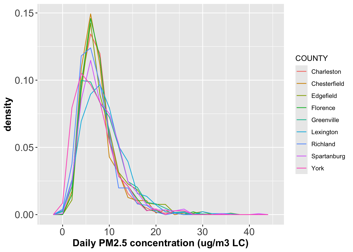
Generate density plots of PM2.5 concentrations grouped by County in one single panel, where each density should have its own color. What do you find from the figure?
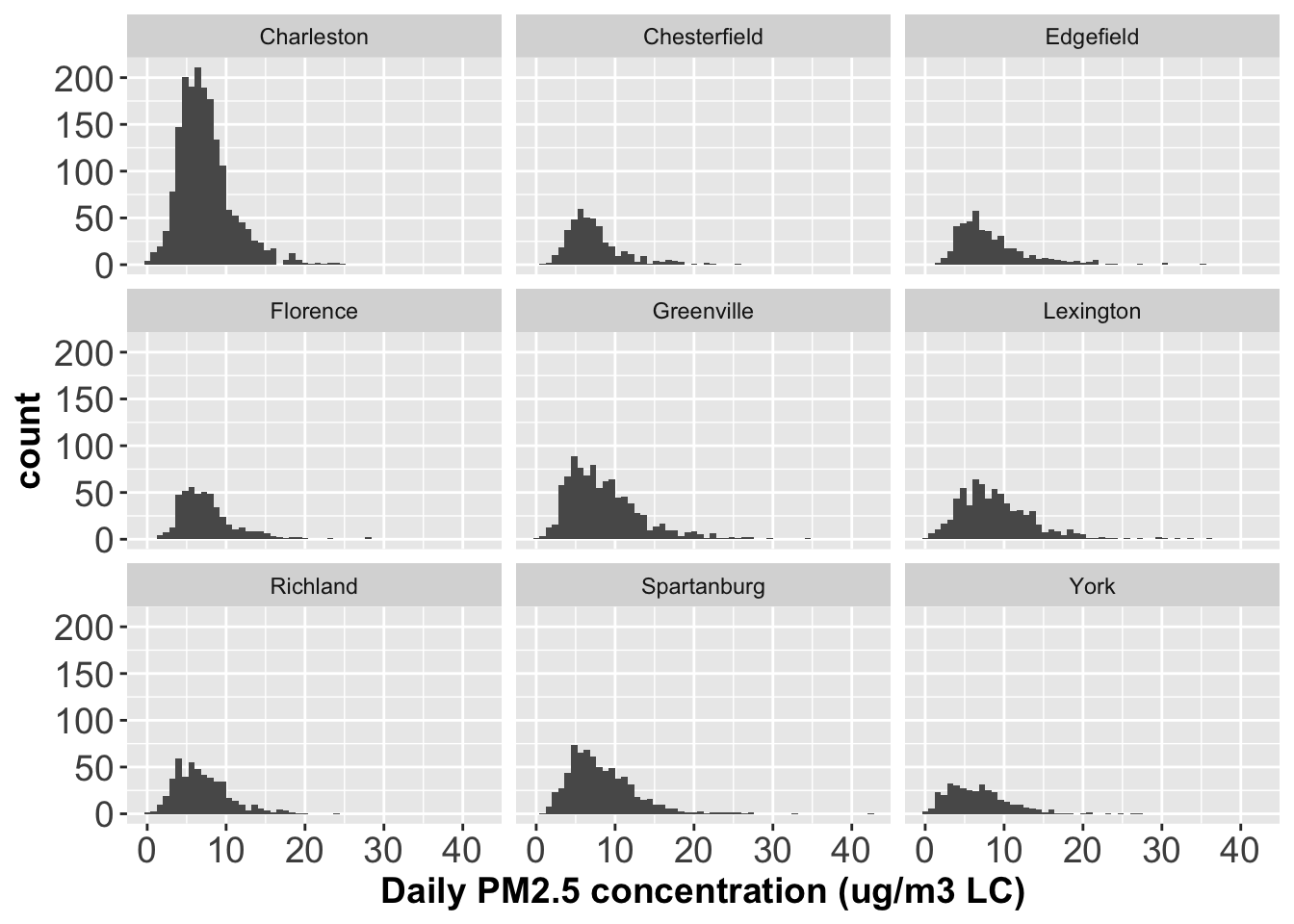
Plot histograms of PM2.5 concentrations across different counties with one panel for one histogram.
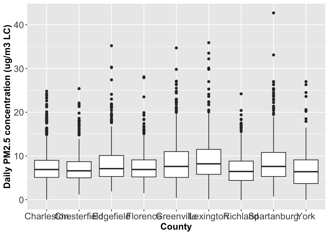
Generate boxplots of PM2.5 concentrations by County. What would you say about the distributions?
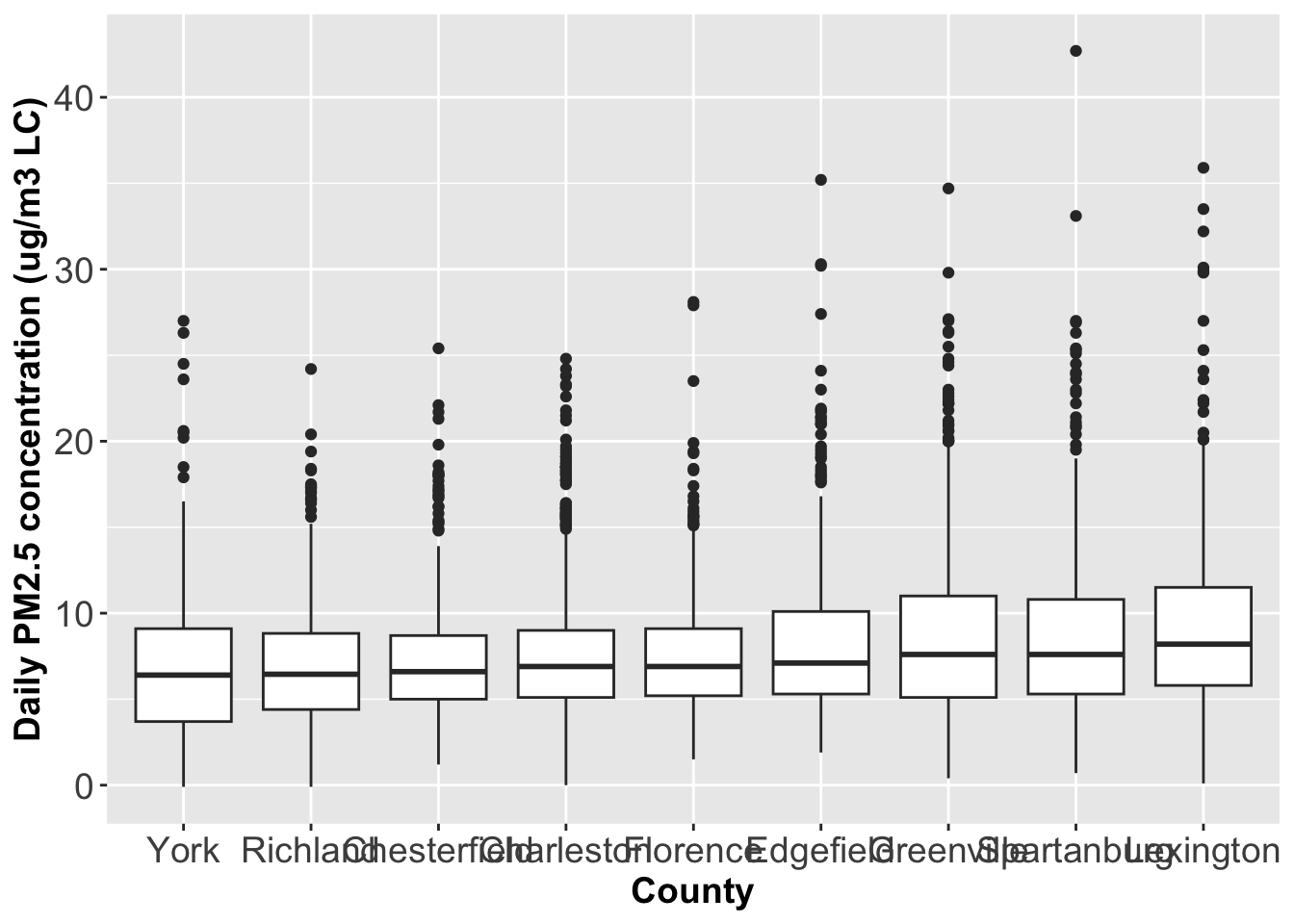
Reorder the boxplots above by the median value of PM2.5 concentrations.
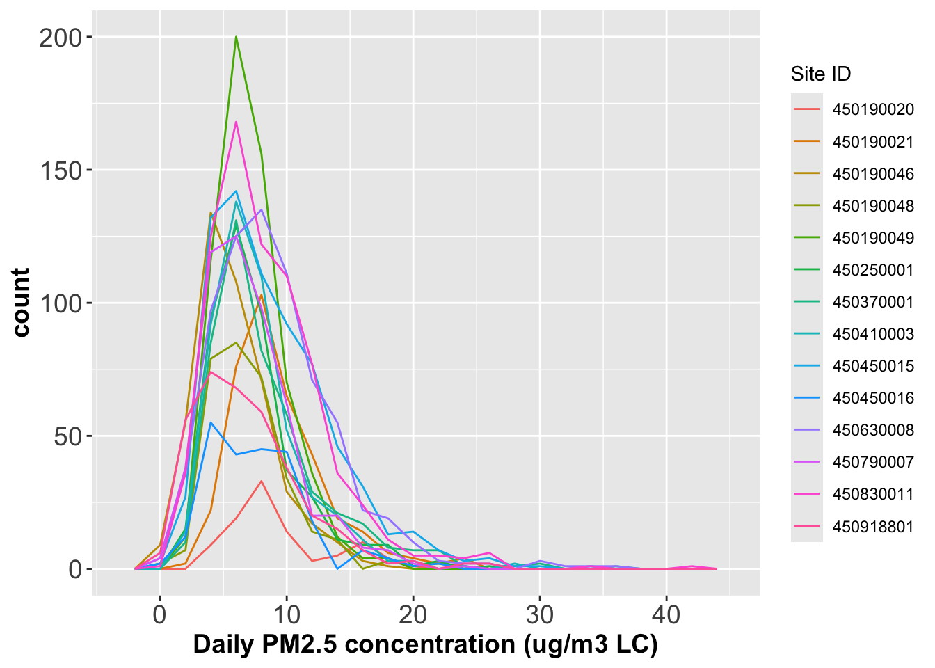
Converting the Site ID to a factor and plot the histogram grouped by Site ID.
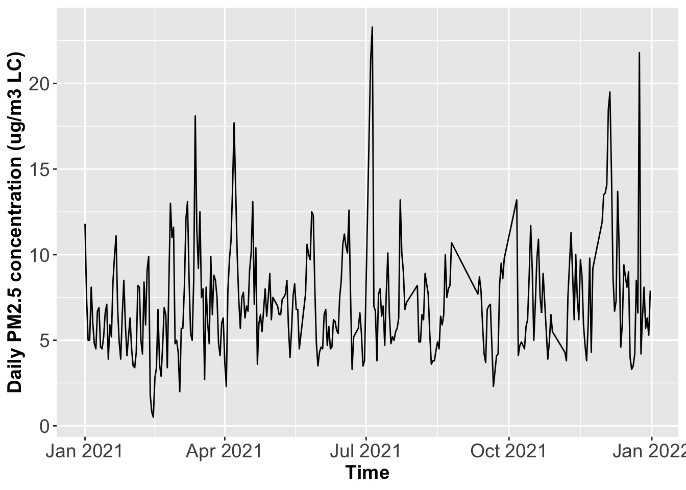
Generate the time series plot for the monitoring Site ID 450190048.
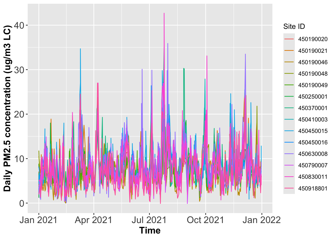
Plot time series of PM2.5 concentrations for all monitoring sites in one panel, where each site has its own color
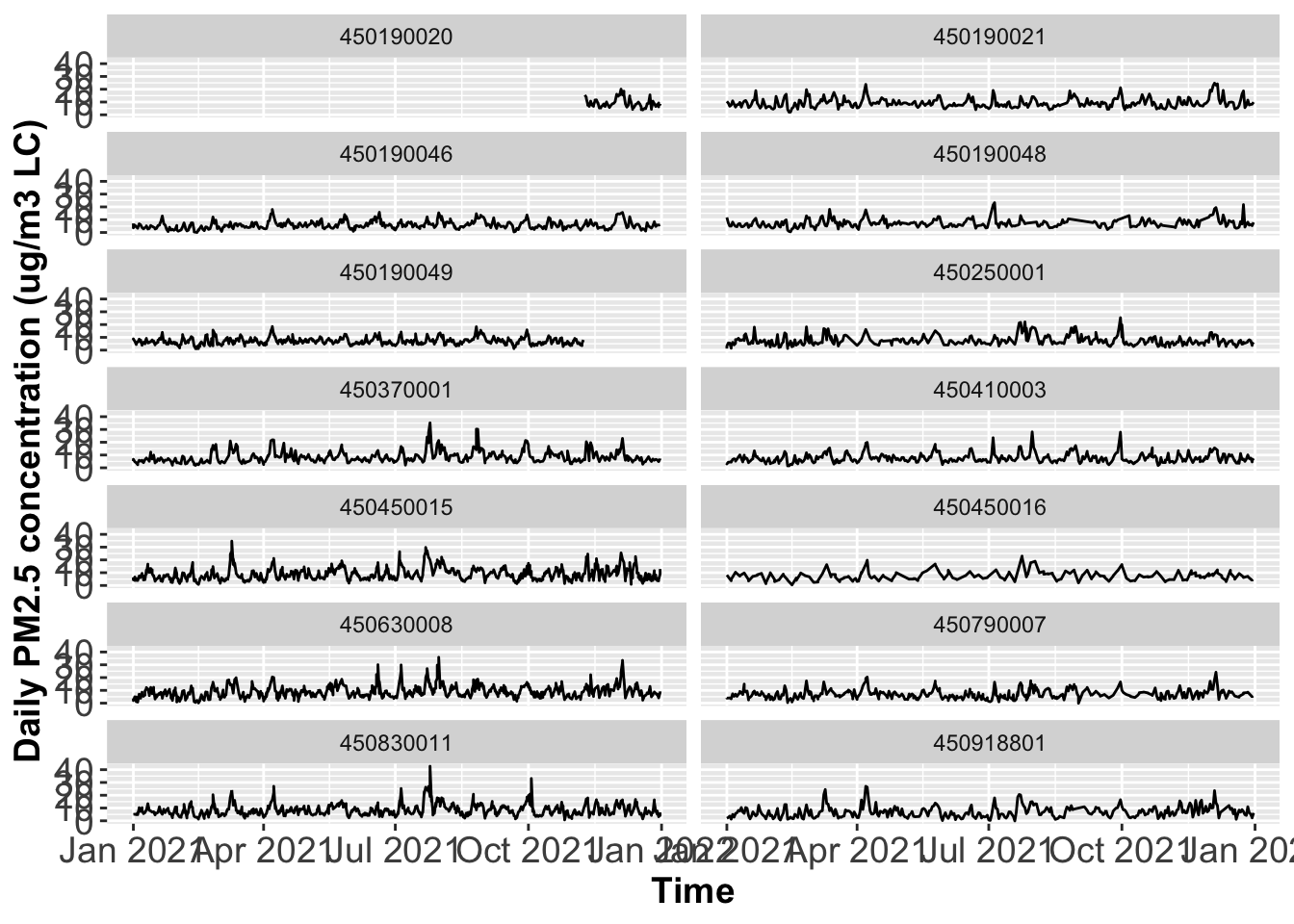
Plot time series of PM2.5 concentrations across all monitoring sites in multiple panels, where one panel only has one site, and each row only has two panels.
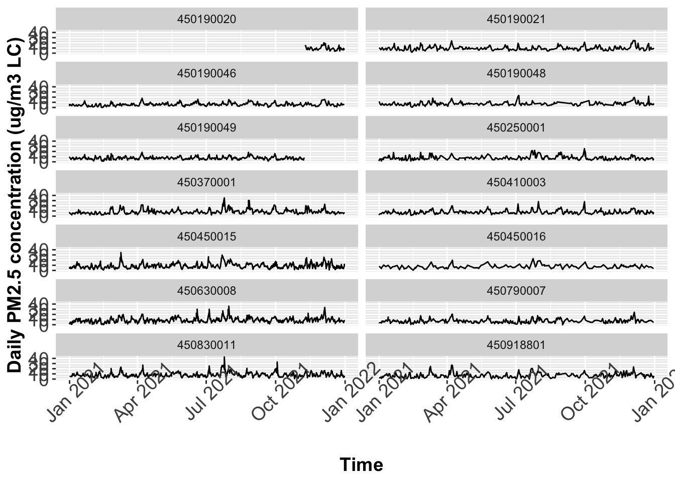
In the time series plot, there seems to be not enough space to hold the x-axis labels. One way to avoid this is to rotate the axis labels. Please rotate all the time labels 45 degree.

View Solution

Code

library(readr)
library(lubridate)

df = read_csv("AQSdata.csv")
head(df)

# A tibble: 6 × 20
  Date       Source `Site ID`   POC Daily Mean PM2.5 Con…¹ UNITS DAILY_AQI_VALUE
  <chr>      <chr>      <dbl> <dbl>                  <dbl> <chr>           <dbl>
1 11/09/2021 AQS    450190020     1                   15.5 ug/m…              58
2 11/10/2021 AQS    450190020     1                   13.6 ug/m…              54
3 11/11/2021 AQS    450190020     1                    8.1 ug/m…              34
4 11/12/2021 AQS    450190020     1                    7.1 ug/m…              30
5 11/13/2021 AQS    450190020     1                   10.7 ug/m…              45
6 11/14/2021 AQS    450190020     1                    7.5 ug/m…              31
# ℹ abbreviated name: ¹`Daily Mean PM2.5 Concentration`
# ℹ 13 more variables: `Site Name` <chr>, DAILY_OBS_COUNT <dbl>,
#   PERCENT_COMPLETE <dbl>, AQS_PARAMETER_CODE <dbl>, AQS_PARAMETER_DESC <chr>,
#   CBSA_CODE <dbl>, CBSA_NAME <chr>, STATE_CODE <dbl>, STATE <chr>,
#   COUNTY_CODE <chr>, COUNTY <chr>, SITE_LATITUDE <dbl>, SITE_LONGITUDE <dbl>

Code

theme_mat = theme(axis.text = element_text(size = 14),
                  axis.title = element_text(size = 14, face = "bold"))
df = rename(df, PM2.5 = `Daily Mean PM2.5 Concentration`)
ggplot(df) +
  geom_freqpoly(aes(
    x = PM2.5,
    y = after_stat(density),
    color = COUNTY
  ), binwidth = 2) +
  xlab("Daily PM2.5 concentration (ug/m3 LC)") +
  theme_mat

Code

ggplot(df) +
  geom_histogram(aes(x = PM2.5), binwidth = .8) +
  facet_wrap(~ COUNTY, ncol = 3) +
  xlab("Daily PM2.5 concentration (ug/m3 LC)") +
  theme_mat

Code

ggplot(df) +
  geom_boxplot(aes(x = COUNTY, y = PM2.5)) +
  xlab("County") +
  ylab("Daily PM2.5 concentration (ug/m3 LC)") +
  theme_mat

Code

ggplot(df) +
  geom_boxplot(aes(x = reorder(COUNTY, PM2.5, FUN = median), 
                   y = PM2.5)) +
  xlab("County") +
  ylab("Daily PM2.5 concentration (ug/m3 LC)") +
  theme_mat

Code

df1 = df
df1$`Site ID` =  as.factor(df$`Site ID`)
ggplot(df1) +
  geom_freqpoly(aes(x = PM2.5, color = `Site ID`), binwidth = 2) +
  xlab("Daily PM2.5 concentration (ug/m3 LC)") +
  theme_mat

Code

df1 %>%
  filter(`Site ID` == 450190048) %>%
  ggplot() +
  geom_line(aes(x = mdy(Date), y = PM2.5)) +
  labs(x = "Time", y = "Daily PM2.5 concentration (ug/m3 LC)") + 
  theme_mat

Code

df1 %>%
  ggplot() +
  geom_line(aes(x = mdy(Date), y = PM2.5, color = `Site ID`)) +
  labs(x = "Time", y = "Daily PM2.5 concentration (ug/m3 LC)") + 
  theme_mat

Code

g <- df1 %>%
  ggplot() +
  geom_line(aes(x = mdy(Date), y = PM2.5)) +
  facet_wrap(~ `Site ID`, ncol = 2) +
  labs(x = "Time", y = "Daily PM2.5 concentration (ug/m3 LC)") + 
  theme_mat
print(g)

Code

g + theme(axis.text.x = element_text(angle = 45))

1.8.5 Exercise 5: Working with `dplyr` Package

Continuing working with the above PM 2.5 data.

Filter all the observations in the county Greenville. How many observations are there?
Filter all the observations in Greenville in August 2021
Filter all the observations in Greenville in August 2021 and select the variables PM2.5 concentrations, Date, latitude and longitude of sites
Generate scatterplots of PM2.5 against latitude and longitude in two different panels

View Solution

Code

library(dplyr)

df %>%
  filter(COUNTY == "Greenville")

# A tibble: 937 × 20
   Date       Source `Site ID`   POC PM2.5 UNITS    DAILY_AQI_VALUE `Site Name` 
   <chr>      <chr>      <dbl> <dbl> <dbl> <chr>              <dbl> <chr>       
 1 01/01/2021 AQS    450450015     1   6.3 ug/m3 LC              26 Greenville …
 2 01/02/2021 AQS    450450015     1   6.6 ug/m3 LC              28 Greenville …
 3 01/03/2021 AQS    450450015     1   5.4 ug/m3 LC              23 Greenville …
 4 01/05/2021 AQS    450450015     1   7.4 ug/m3 LC              31 Greenville …
 5 01/06/2021 AQS    450450015     1   7.7 ug/m3 LC              32 Greenville …
 6 01/07/2021 AQS    450450015     1   9.5 ug/m3 LC              40 Greenville …
 7 01/08/2021 AQS    450450015     1   7.5 ug/m3 LC              31 Greenville …
 8 01/09/2021 AQS    450450015     1   5.3 ug/m3 LC              22 Greenville …
 9 01/10/2021 AQS    450450015     1  12.1 ug/m3 LC              51 Greenville …
10 01/11/2021 AQS    450450015     1  16.7 ug/m3 LC              61 Greenville …
# ℹ 927 more rows
# ℹ 12 more variables: DAILY_OBS_COUNT <dbl>, PERCENT_COMPLETE <dbl>,
#   AQS_PARAMETER_CODE <dbl>, AQS_PARAMETER_DESC <chr>, CBSA_CODE <dbl>,
#   CBSA_NAME <chr>, STATE_CODE <dbl>, STATE <chr>, COUNTY_CODE <chr>,
#   COUNTY <chr>, SITE_LATITUDE <dbl>, SITE_LONGITUDE <dbl>

Code

df %>%
  mutate(Date = mdy(Date), YM = format_ISO8601(Date, precision = "ym")) %>%
  filter(COUNTY == "Greenville", YM == "2021-08")

# A tibble: 82 × 21
   Date       Source `Site ID`   POC PM2.5 UNITS    DAILY_AQI_VALUE `Site Name` 
   <date>     <chr>      <dbl> <dbl> <dbl> <chr>              <dbl> <chr>       
 1 2021-08-01 AQS    450450015     1  13.8 ug/m3 LC              55 Greenville …
 2 2021-08-02 AQS    450450015     1  19   ug/m3 LC              66 Greenville …
 3 2021-08-03 AQS    450450015     1  16.9 ug/m3 LC              61 Greenville …
 4 2021-08-04 AQS    450450015     1  15.6 ug/m3 LC              58 Greenville …
 5 2021-08-05 AQS    450450015     1  11   ug/m3 LC              46 Greenville …
 6 2021-08-06 AQS    450450015     1  10.3 ug/m3 LC              43 Greenville …
 7 2021-08-07 AQS    450450015     1   9.7 ug/m3 LC              40 Greenville …
 8 2021-08-08 AQS    450450015     1  10   ug/m3 LC              42 Greenville …
 9 2021-08-09 AQS    450450015     1  12   ug/m3 LC              50 Greenville …
10 2021-08-10 AQS    450450015     1  12.5 ug/m3 LC              52 Greenville …
# ℹ 72 more rows
# ℹ 13 more variables: DAILY_OBS_COUNT <dbl>, PERCENT_COMPLETE <dbl>,
#   AQS_PARAMETER_CODE <dbl>, AQS_PARAMETER_DESC <chr>, CBSA_CODE <dbl>,
#   CBSA_NAME <chr>, STATE_CODE <dbl>, STATE <chr>, COUNTY_CODE <chr>,
#   COUNTY <chr>, SITE_LATITUDE <dbl>, SITE_LONGITUDE <dbl>, YM <chr>

Code

df %>%
  mutate(Date = mdy(Date), YM = format_ISO8601(Date, precision = "ym")) %>%
  filter(COUNTY == "Greenville", YM == "2021-08") %>%
  dplyr::select(PM2.5, Date, SITE_LATITUDE, SITE_LONGITUDE)

# A tibble: 82 × 4
   PM2.5 Date       SITE_LATITUDE SITE_LONGITUDE
   <dbl> <date>             <dbl>          <dbl>
 1  13.8 2021-08-01          34.8          -82.4
 2  19   2021-08-02          34.8          -82.4
 3  16.9 2021-08-03          34.8          -82.4
 4  15.6 2021-08-04          34.8          -82.4
 5  11   2021-08-05          34.8          -82.4
 6  10.3 2021-08-06          34.8          -82.4
 7   9.7 2021-08-07          34.8          -82.4
 8  10   2021-08-08          34.8          -82.4
 9  12   2021-08-09          34.8          -82.4
10  12.5 2021-08-10          34.8          -82.4
# ℹ 72 more rows

Code

df %>%
  dplyr::select(PM2.5, SITE_LATITUDE, SITE_LONGITUDE) %>%
  pivot_longer(
    cols = c("SITE_LATITUDE", "SITE_LONGITUDE"),
    names_to = "variable",
    values_to = "value"
  ) %>%
  ggplot(aes(x = value, y = PM2.5)) +
  geom_point() +
  facet_wrap( ~ variable, scale = "free") +
  xlab("") +
  ylab("Daily PM2.5 concentration (ug/m3 LC)") +
  theme_mat

1.1 Course Outline

1.2 Objectives of Multivariate Analysis

1.3 Introduction to R and RStudio

1.3.1 Getting Started

1.3.2 Introduction to R Programming

1.4 Organization of Data and Notation

1.5 Descriptive Statistics

1.5.1 Sample Mean

1.5.2 Sample Variance and Sample Standard Deviation

1.5.3 Sample Covariance and Sample Correlation

1.5.4 Covariance and Correlation Measures

1.6 Matrix Organization of Descriptive Statistics

1.6.1 Sample Mean

1.6.2 Sample Covariance

1.6.3 Sample Correlation

1.7 Standardization

1.7.1 Standardized Data (or z-Scores)

1.7.2 Standardized Population Mean

1.7.3 Standardized Population Covariance

1.8 Exercises

1.8.1 Exercise 1: Data Types

1.8.2 Exercise 2: Working with Matrix and Data Frames

1.8.3 Exercise 3: Linear Algebra

1.8.4 Exercise 4: Working with ggplot2 Package

1.8.5 Exercise 5: Working with dplyr Package

1.8.4 Exercise 4: Working with `ggplot2` Package

1.8.5 Exercise 5: Working with `dplyr` Package